1. Reference problem#

1.1. Geometry#

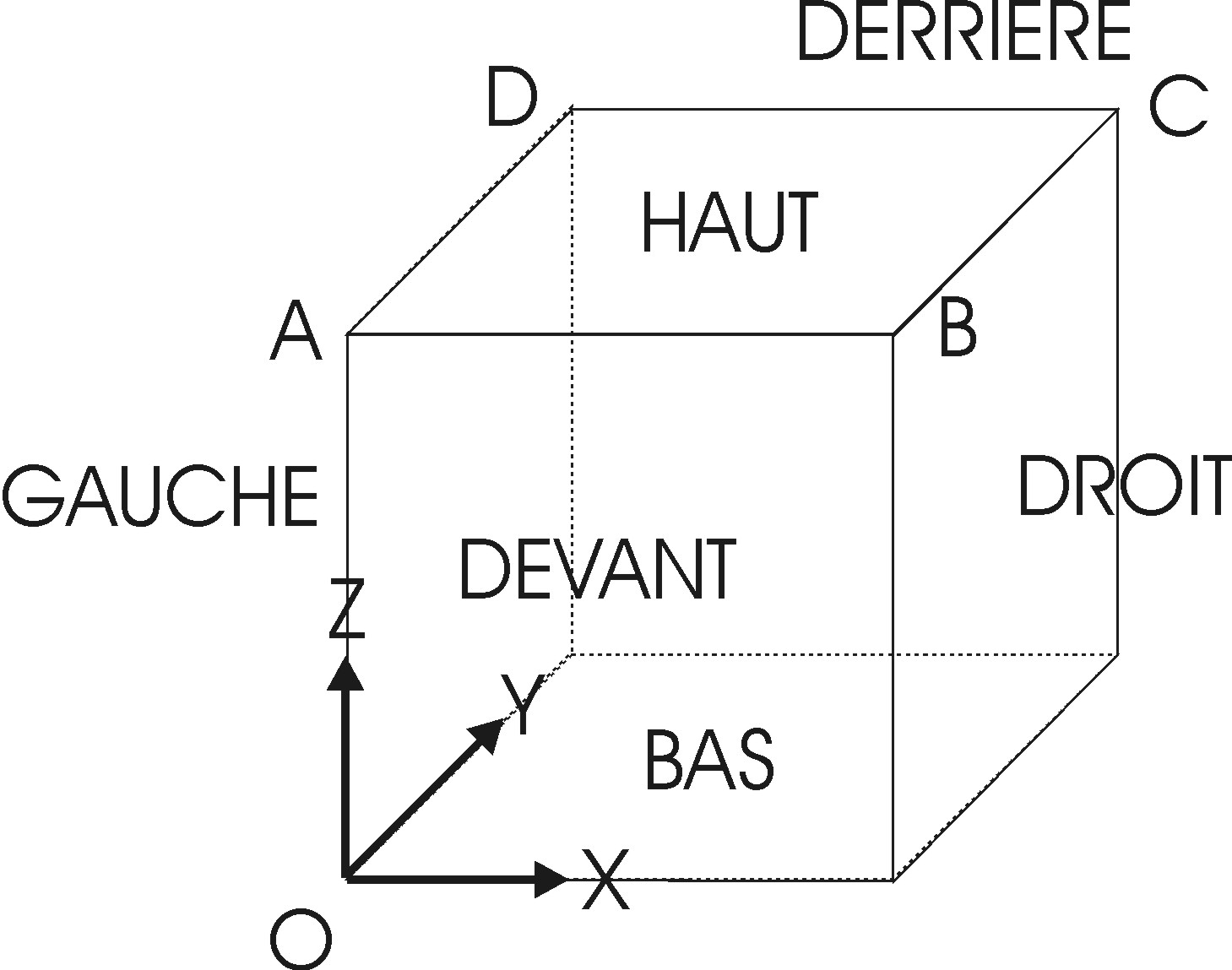
The triaxial test is carried out on a single isoparametric finite element of cubic shape \(\mathrm{CUB8}\). The length of each edge is 1. The different facets of this cube are mesh groups named \(\mathrm{HAUT}\), \(\mathrm{BAS}\),, \(\mathrm{DEVANT}\), \(\mathrm{DERRIERE}\), \(\mathrm{DROIT}\), and \(\mathrm{GAUCHE}\). The mesh group SYM also contains the mesh groups \(\mathrm{BAS}\), \(\mathrm{DEVANT}\) and \(\mathrm{GAUCHE}\); the group of elements \(\mathrm{COTE}\) the mesh groups \(\mathrm{DERRIERE}\) and \(\mathrm{DROIT}\).

1.2. Material properties#

The elastic properties are:

- isotropic compressibility module: \(K=516200\mathrm{kPa}\)
- shear modulus: \(\mu =238200\mathrm{kPa}\)

The anelastic properties (Humjeux) are:

- power of the nonlinear elastic law: \({n}_{e}=0.4\)
- \(\beta =24\)
- \(d=2.5\)
- \(b=0.2\)
- friction angle: \(\varphi =33°\)
- angle of expansion: \(\psi =33°\)
- critical pressure: \({P}_{\mathrm{c0}}=-1000\mathrm{kPa}\)
- reference pressure: \({P}_{\mathrm{ref}}=-1000\mathrm{kPa}\)
- elastic radius of the isotropic mechanism: \({r}_{\mathrm{éla}}^{s}=0.001\)
- elastic radius of the deviatory mechanism: \({r}_{\mathrm{éla}}^{d}=0.005\)
- \({a}_{\mathrm{mon}}=0.0001\)
- \({a}_{\mathrm{cyc}}=0.008\)
- \({c}_{\mathrm{mon}}=0.2\)
- \({c}_{\mathrm{cyc}}=0.1\)
- \({r}_{\mathrm{hys}}=0.05\)
- \({r}_{\mathrm{mob}}=0.9\)
- \({x}_{m}=1\)
- \(\text{dila}=1\)

1.3. Boundary conditions and loads#

A triaxial test consists in imposing on the specimen a variation in vertical load while maintaining the lateral pressure constant. It can be drained (the interstitial fluid pressure does not vary during the test) or non-drained (the tap is closed: the fluid interstitial pressure changes in the sample). We are interested here in the drained case, which is simpler, because it does not involve the influence of the interstitial pressure of the fluid and can therefore be modelled by a pure mechanical calculation.

In the model under consideration, the cubic element represents one eighth of the sample. The boundary conditions are therefore as follows:

- - Symmetry conditions:
    \({u}_{z}=0\) on mesh group \(\mathrm{BAS}\)
    
    \({u}_{x}=0\) on mesh group \(\mathrm{GAUCHE}\)
    
    \({u}_{y}=0\) on mesh group \(\mathrm{DEVANT}\)
  - Lateral pressure conditions:
    \({P}_{n}=1\) on mesh group \(\mathrm{COTE}\)
  - Loading conditions:
    \({P}_{n}=1\) on mesh group \(\mathrm{HAUT}\) (phase 1)
    
    \({u}_{z}=-1\) on mesh group \(\mathrm{HAUT}\) (phase 2)

Charging is carried out in two phases:

- isotropic loading between \(t=-2\) and \(t=0\) where the pressure on the cell groups \(\mathrm{COTE}\) and HAUT varies between \(p=0\) and \(p={p}_{c}\) (isotropic preconsolidation pressure). In models A, B, and C, the value of \({p}_{c}\) is \(\mathrm{50,}\mathrm{100,}200\mathrm{kPa}\) respectively;
- displacement imposed on the group of elements \(\mathrm{HAUT}\) and varying between \(t=0\) and \(t=10\) from \({u}_{z}=0\) and \({u}_{z}=-0.2\) (total vertical deformation of \(20\text{\%}\)).

1.4. Results#

The solutions are post-treated at point \(C\), in terms of equivalent stress \(Q\), total volume deformation \({\varepsilon }_{v}\) and isotropic work-hardening coefficients \(({r}_{\text{ela}}^{\text{s},m}+{r}_{\text{iso}}^{m})\) and deviation \(({r}_{\text{ela}}^{d,m}+{r}_{\text{dev}}^{m})\), according to the evolution of the axial deformation \({\epsilon }_{\mathit{zz}}\)

Validation is carried out by comparison with GEFDYN solutions provided by École Centrale Paris.

For models that promote the large deformations approach with the operator GDEF_LOG, we consider the logarithmic deformation \(\underline{\underline{E}}=1/2\mathrm{log}(I+2\underline{\underline{\Lambda }})\), with \(\underline{\underline{\Lambda }}\) the Green-Lagrange tensor. The volume deformation in this case is directly obtained from the deformation gradient determinant, \(J=\mathit{det}(F)\).