5. D modeling

5.1. Characteristics of modeling

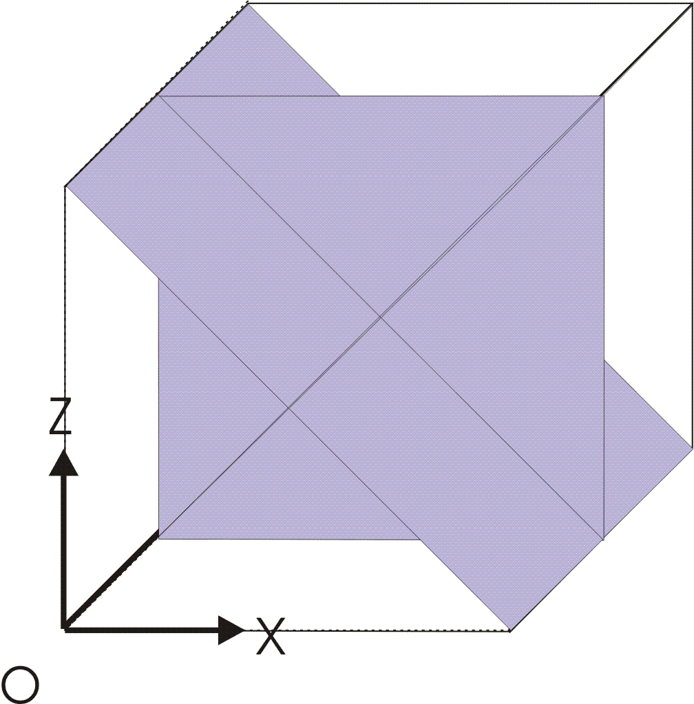
The aim of this modeling is to test the functionality of reorienting the local coordinate system defining the three sliding planes linked to the deviatory mechanisms of Hujeux’s law. This reorientation is carried out using the AFFE_CARA_ELEM® MASSIF operator.

D modeling is*three-dimensional and*static nonlinear*.

We first perform an elastic preconsolidation (\(\mathrm{ELAS}\)) of the sample up to \({p}_{c}=100\mathrm{kPa}\) (1st phase of the calculation). This preconsolidation takes place in \(1\), a time step between \(t=-2\) and \(t=0\).

The vertical displacement imposed on the upper facet varies between \(0.\) and \(-0.2\) (2nd phase of the calculation) in 100 steps of time between \(t=0\) and \(t=10\). During this second phase, the automatic subdivision of the time step is activated to manage situations of non-convergence of local integration.

We test the reorientation of the sliding planes defined by a rotation of the coordinate system of \(45°\) around the axis (\(\mathit{OZ}\)). This reorientation is defined by AFFE_CARA_ELEM® MASSIF.

We load the object CARAEL defining the orientation of the local coordinate system on which the sliding planes of Hujeux’s law will be defined. In the integration of equilibrium equations, an update of the tangent matrix is required, which is provided by the routines of Hujeux’s law and significantly accelerates convergence. We also require the subdivision of the time step (command DEFI_LIST_INST) to deal with situations where local integration fails due to excessively large load increments. This feature is highly recommended.

5.2. Quantities tested and results of modeling D

5.2.1. Tested values

The solutions are calculated at point \(C\) and compared to an identical calculation performed (with Code_Aster) on a sample previously rotated from \(45°\). They are given in terms of equivalent stress \(Q\), total volume deformation \({\varepsilon }_{v}\) and isotropic work-hardening coefficients \(({r}_{\text{ela}}^{\text{iso},m}+{r}_{\text{iso}}^{m})\) and deviatory \(({r}_{\text{ela}}^{d,m}+{r}_{\text{dev}}^{m})\), and summarized in the following tables:

\(Q=\sqrt{\frac{1}{2}\underline{\underline{s}}\mathrm{:}\underline{\underline{s}}}[\mathit{Pa}]\)

\({\varepsilon }_{\mathit{zz}}\)	Code_Aster	GEFDYN	relative error
-2%	148396	148396	0.0002%
-4%	176513	176513	0.006%
-6%	185559	185554	0.002%
-8%	187683	187681	0.001%
-10%	186806	186804	0.001%

\({\epsilon }_{V}\mathrm{=}\text{trace}(\epsilon )\)

\({\varepsilon }_{\mathit{zz}}\)	Code_Aster	GEFDYN	relative error
-2%	-7.40E-3	-7.40E-3	0.001%
-4%	-6.72E-3	-6.72E-3	0.016%
-6%	-4.36E-3	-4.36E-3	-0.001%
-8%	-1.45E-3	-1.45E-3	-0.013%
-10%	1.63E-3	1.63E-3	0.018%

\(({r}_{\text{ela}}^{d,m}+{r}_{\text{dev}}^{m})\)

\({\varepsilon }_{\mathit{zz}}\)	Code_Aster	GEFDYN	relative error
-2%	0.565	0.565	-0.062%
-4%	0.630	0.630	0.008%
-6%	0.654	0.654	0.073%
-8%	0.666	0.666	-0.035%
-10%	0.671	0.671	0.054%

\(({r}_{\text{ela}}^{\text{iso},m}+{r}_{\text{iso}}^{m})\)

\({\varepsilon }_{\mathit{zz}}\)	Code_Aster	GEFDYN	relative error
-2%	0.067	0.067	-0.564%
-4%	0.074	0.074	0.140%
-6%	0.081	0.081	-0.499%
-8%	0.087	0.087	-0.038%
-10%	0.093	0.093	0.093	0.421%

5.2.2. Comments

The relative error is always very small, which is normal, since it is ultimately exactly the same calculation.