1. Reference problem#
1.1. Geometry#
The 3D structure with dimensions \(\mathit{LX}\mathrm{=}\mathrm{1m}\), \(\mathit{LY}\mathrm{=}\mathrm{2m}\) and \(\mathit{LZ}\mathrm{=}\mathrm{3m}\) includes a flat horizontal interface located halfway up (see [Figure 1.1-1]).
The interface is not meshed, and the geometry is in fact a healthy structure without an interface. The interface is then introduced by level sets directly into the command file using the DEFI_FISS_XFEM [U4.82.08] operator.

Figure 1.1-1 : 3D structure geometry
We define the points \(A\), \(B\), \(C\),, \(D\),, \(E\) and \(F\) which will be used to block rigid modes.
\(x\) |
|
|
|
\(A\) |
LX |
\(\mathrm{LY}/2\) |
|
\(B\) |
|
|
|
\(C\) |
|
|
|
\(D\) |
|
|
LZ |
\(E\) |
|
|
LZ |
\(F\) |
|
|
LZ |
Table 1.1-1 : Coordinates of blocking points in 3D
The equivalent structure is also defined in 2D, with dimensions \(\mathrm{LX}=\mathrm{2m}\), \(\mathrm{LY}=\mathrm{3m}\) with a flat horizontal interface located halfway up (see [Figure 1.1-2]).
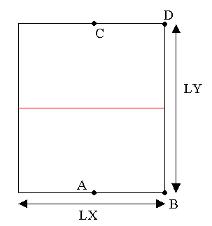
Figure 1.1-2 : 2D Structure Geometry
We define the points \(A\), \(B\), \(C\) and \(D\) that will be used to block rigid modes.
\(x\) |
|
|
\(A\) |
|
|
\(B\) |
|
|
\(C\) |
|
|
\(D\) |
|
|
Table 1.1-2 : Coordinates of blocking points in 2D
1.2. Material properties#
Young’s module: \(E=10000\mathrm{MPa}\)
Poisson’s ratio: \(\nu =0\)
1.3. Boundary conditions and loads#
In 3D, rigid modes are blocked in the following way:
|
\(\{\begin{array}{}{\mathrm{DX}}^{A}={\mathrm{DX}}^{D}=0\\ {\mathrm{DY}}^{A}={\mathrm{DY}}^{D}=0\\ {\mathrm{DZ}}^{A}={\mathrm{DZ}}^{D}=0\end{array}\) |
|
\({\mathrm{DZ}}^{B}={\mathrm{DZ}}^{E}=0\) |
|
\(\{\begin{array}{}{\mathrm{DX}}^{C}={\mathrm{DX}}^{F}=0\\ {\mathrm{DZ}}^{C}={\mathrm{DZ}}^{F}=0\end{array}\) |
In 2D, rigid modes are blocked in the following way:
|
\(\{\begin{array}{}{\mathrm{DX}}^{A}={\mathrm{DX}}^{C}=0\\ {\mathrm{DY}}^{A}={\mathrm{DY}}^{C}=0\end{array}\) |
|
\({\mathrm{DY}}^{B}={\mathrm{DY}}^{D}=0\) |
In 3D, two loads are envisaged:
Constant distributed pressure (\(p=10000\mathrm{Pa}\)) on the lateral faces (planes \(y=0\) and \(y=\mathrm{LY}\)), corresponding to a case of compression along the axis \(\mathrm{Oy}\).
Positive pressure (\(p=10000\mathrm{Pa}\)) on the upper lateral faces and a negative pressure (\(p=-10000\mathrm{Pa}\)) on the lower lateral faces, corresponding to a case of compression on the upper solid and a case of tension on the lower solid
In 2D, two loads are envisaged:
Constant distributed pressure (\(p=10000\mathrm{Pa}\)) on the lateral segments (\(x=0\) and \(x=\mathrm{LX}\)), corresponding to a case of compression along the \(\mathrm{Ox}\) axis.
Positive pressure (\(p=10000\mathrm{Pa}\)) on the upper lateral edges and a negative pressure (\(p=-10000\mathrm{Pa}\)) on the lower lateral edges, corresponding to a case of compression on the upper solid and a case of tension on the lower solid

Figure 1.3-1 : Pressure loading
1.4. Problem solutions#
The solution to the 3D problem is presented. That of the 2D problem is obtained by replacing \(y\) by \(x\).
1.4.1. Pure compression loading#
The structure is in pure compression, the solution on the go is trivial. For the nodes on the left lateral face, the displacement solution is:
\({u}_{y}\mathrm{=}\mathrm{-}\frac{\mathit{LY}}{2}{\varepsilon }_{\mathit{yy}}\mathrm{=}\mathrm{-}\frac{\mathit{LY}}{2}\frac{{\sigma }_{\mathit{yy}}}{E}\mathrm{=}\frac{\mathit{LY}}{2}\frac{p}{E}\mathrm{=}\frac{{2.10}^{4}}{{2.10}^{10}}\mathrm{=}{10}^{\mathrm{-}6}m\)
For the nodes on the right side face, the displacement solution is:
\({u}_{y}\mathrm{=}\frac{\mathit{LY}}{2}{\varepsilon }_{\mathit{yy}}\mathrm{=}\frac{\mathit{LY}}{2}\frac{{\sigma }_{\mathit{yy}}}{E}\mathrm{=}\frac{\mathrm{-}\mathit{LY}}{2}\frac{p}{E}\mathrm{=}\mathrm{-}\frac{{2.10}^{4}}{{2.10}^{10}}\mathrm{=}\mathrm{-}{10}^{\mathrm{-}6}m\)
When an edge node is enriched by the Heaviside function, its displacement is written as a combination of a continuous term and a discontinuous term. For this load case, there is no discontinuity across the interface, so the enriched degrees of freedom are all zero.
1.4.2. Compression/traction loading#
The upper structure is in pure compression and the movements of the nodes on the upper lateral face are the same as those of the previous load case.


The lower structure is in pure traction. Only the signs of the displacement values change. For the nodes on the lower left side, the displacement solution is:
\({u}_{y}=-\frac{\mathrm{LY}}{2}{\varepsilon }_{\mathrm{yy}}=\frac{\mathrm{LY}}{2}\frac{p}{E}=-\frac{{2.10}^{4}}{{2.10}^{10}}=-{10}^{-6}m\)
For the nodes on the lower right side, the displacement solution is:
\({u}_{y}=\frac{\mathrm{LY}}{2}{\varepsilon }_{\mathrm{yy}}=\frac{\mathrm{LY}}{2}\frac{p}{E}=\frac{{2.10}^{4}}{{2.10}^{10}}={10}^{-6}m\)
In this case, the movement is discontinuous across the interface. The values of discontinuous degrees of freedom can be easily determined (we will refer to the similar case treated in [V6.04.173]).