2. Modeling A#
The list of moments is used to control the Norton-Hoff regularization method by means of a coefficient \(t\), (\(m=1+{\text{10}}^{1-t}\)), and not the evolution of the load as during an ordinary calculation.
To perform a calculation in code_aster in limit analysis with the Norton-Hoff-Friaâ regularization method with the vonMises resistance criterion, it is necessary:
define the 2D (plane or axis) or 3D model with the almost incompressible finite elements, 3D models_ INCO_UPG, D_ PLAN_INCO_UPG, or AXIS_INCO_UPG;
ensure the incompressibility condition: GONF =0 in AFFE_CHAR_MECA;
define only the characteristic of the material \({s}_{y}\), the limit load being independent of

and \(\mathrm{\nu }\);
define the permanent load and the one set by \(\lambda\);
define discretization in time, (in practice between \({t}_{\mathit{min}}=1\) and \({t}_{\mathit{max}}=2\) to \(5\));
perform a non-linear calculation with the behavior relationship NORTON_HOFF with the command STAT_NON_LINE [U4.51.03], and the control ANA_LIM. In practice, linear research can be used to improve convergence and the subdivision of the time step;
post-process the calculation to get the load limit with the POST_ELEM [U4.81.22] command.
2.1. Characteristics of modeling#
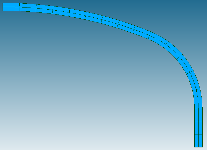
We consider a cylinder modelled by incompressible axisymmetric elements of type QUAD8.
2.2. Characteristics of the mesh#
Number of knots: 141
|
|
2.3. Tested sizes and results#
With the mesh in question, the calculation of the test case is stopped at \(t=\mathrm{2,450}s\). Additional details on the calculation are provided in the user support document [U2.05.04].
The Norton-Hoff coefficient corresponding to this moment is \(m=\mathrm{1,0355}\).
The table below shows the extraction of the values of \(\mathrm{\lambda }\) at certain times when the calculation is stopped, as well as the comparison with the reference values.
Modeling |
Estimated upper value |
Estimated lower value |
||
EDF |
\(t=2\) |
\(m=\mathrm{1,1}\) |
\(\mathrm{3,94863}\) |
\(\mathrm{3,27091}\) |
\(t=\mathrm{2,125}\) |
\(m=\mathrm{1,0750}\) |
\(\mathrm{3,93504}\) |
\(\mathrm{3,40992}\) |
|
\(t=\mathrm{2,25}\) |
\(m=\mathrm{1,0562}\) |
\(\mathrm{3,92505}\) |
\(\mathrm{3,52215}\) |
|
\(t=\mathrm{2,450}\) |
\(m=\mathrm{1,0355}\) |
\(\mathrm{3,91429}\) |
\(\mathrm{3,65061}\) |
|
Univ. of Liège/ LTAS |
\(\mathrm{3,931}\) |
nought |
||
Research Center FZJ |
nought |
\(\mathrm{3,997}\) |
||
Value tested |
Reference - SOURCE_EXTERNE |
Accuracy |
CHAR_LIMI_SUPà \(t=2\) |
|
|