1. Reference problem#
1.1. Geometry#
The structure is composed of a cylindrical ring crossed by a circular X- FEM interface. Radius \({R}_{2}\) defines the radius of the circular interface (Figure 1.1-1) where contact will be defined.
The characteristic dimensions of the structure are:
\({R}_{1}=\mathrm{1,0}m;{R}_{2}=\mathrm{0,6}m\)
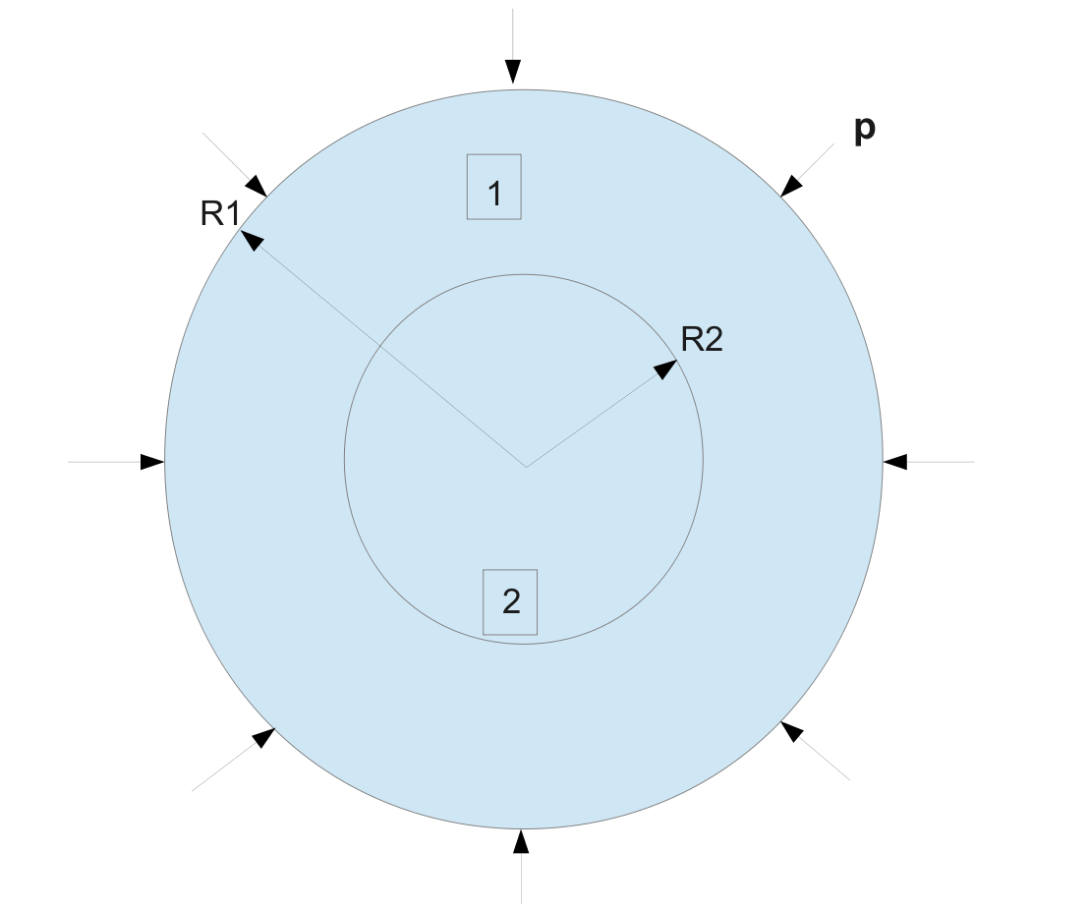
Figure 1.1-a : Structure geometry
1.2. Material properties#
The Young’s modulus and the Poisson’s ratio of the material in the outer ring are given by \({E}_{1}\) and \({\nu }_{1}\) (respectively \({E}_{2}\) and \({\nu }_{2}\) for the inner ring).
1.3. Boundary conditions and loads#
In what follows, the case of a solid disk subjected to a non-uniform external pressure is treated. However, the boundary conditions (as well as the analytical solution) are generalizable to the case of the square surface crossed by a circular interface. The case of the square surface allows us to treat a mesh that would not have the same symmetries as the interface: in the case of the disk, we use a regular radiating mesh, while in the case of the square, we use a regular mesh along the edges of the square.
The application of a non-uniform pressure on the edge \(r={R}_{1}\) of the outer ring is modelled as follows: \(p={\alpha }_{0}+{\alpha }_{1}\mathrm{.}\mathrm{cos}(2\theta )\), \(\theta\) being the polar angle describing the position of the point \(\theta =\mathrm{arctan}(\frac{Y}{X})\). For the analytical calculation, we first solve the problem for a pressure \(p={\alpha }_{0}\), then we solve the problem for a pressure of the form \(p={\alpha }_{1}\mathrm{.}\mathrm{cos}(2\theta )\). For the complete solution, the superposition principle is applied.
Conditions are imposed at the Dirichlet limits. Travel is imposed on the outside surface in \(r={R}_{1}\). We will also define a radius \({R}_{3}=\mathrm{0.2m}\) where we impose displacements, equivalent to those that a full disk would produce (Figure 1.3-1).
For the square area, displacements will be imposed on the outer faces, as well as on the disk with radius \({R}_{3}=\mathrm{0.2m}\).
For each modeling, two calculations are carried out: a first calculation with contact at the interface level, and a second calculation with contact pressure applied at the interface level.
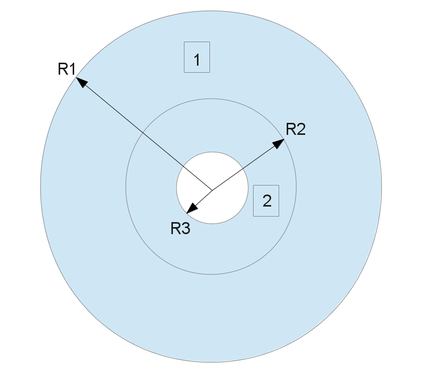
Figure 1.3-a : Structure geometry
1.3.1. Boundary conditions in the case of uniform pressure#
The edges of the solids are subjected to displacements (\(r={R}_{1}\) and \(r={R}_{3}\)) equivalent to the application of pressure \(p={\alpha }_{0}\) on the edge of the outer ring (\(r={R}_{1}\)).
\(\begin{array}{c}{\xi }_{X}(r)=f(r)\mathrm{cos}(\mathrm{arctan}(\frac{Y}{X}))\\ {\xi }_{Y}(r)=f(r)\mathrm{sin}(\mathrm{arctan}(\frac{Y}{X}))\end{array}\)
The function \(f(r)\) of the radial displacement is given as a function of the properties of the materials and the pressure \(p\). In the case of plane deformations (MODELISATION = “D_ PLAN “) we have:
\(\begin{array}{c}f({R}_{1})={A}_{1}{R}_{1}+\frac{{B}_{1}}{{R}_{1}}\\ f({R}_{3})={A}_{2}{R}_{3}\end{array}\) eq 1.1
with:
\(\begin{array}{c}{A}_{1}=\frac{(1+{\nu }_{1})(1-2{\nu }_{1})}{{E}_{1}}\frac{-p{R}_{1}^{2}+\lambda {R}_{2}^{2}}{{R}_{1}^{2}-{R}_{2}^{2}};{B}_{1}=\frac{1+{\nu }_{1}}{{E}_{1}}(-p+\lambda )\frac{{R}_{1}^{2}{R}_{2}^{2}}{{R}_{1}^{2}-{R}_{2}^{2}}\\ {A}_{2}=\frac{-(1+{\nu }_{2})(1-2{\nu }_{2})}{{E}_{2}}\lambda \end{array}\) eq 1.2
where \(\lambda\) is the contact pressure whose analytic expression is:
\(\lambda =2p\frac{(1-{\nu }_{1}^{2})}{{E}_{1}}\frac{\frac{{R}_{1}^{2}}{{R}_{1}^{2}-{R}_{2}^{2}}}{\frac{1+{\nu }_{1}}{{E}_{1}}\frac{{R}_{1}^{2}+{R}_{2}^{2}(1-2{\nu }_{1})}{{R}_{1}^{2}-{R}_{2}^{2}}+\frac{1+{\nu }_{2}}{{E}_{2}}(1-2{\nu }_{2})}\) eq. 1.3
1.3.2. Boundary conditions in the case of variable pressure#
The edges of the rings are subjected to displacements (\(r={R}_{1}\) and \(r={R}_{3}\)) equivalent to the application of pressure \(p={\alpha }_{1}\mathrm{.}\mathrm{cos}(2\theta )\) on the edge of the outer ring (\(r={R}_{1}\)).
\(\begin{array}{c}{\xi }_{X}(r,\theta )={u}_{r}(r,\theta )\mathrm{cos}(\theta )-{u}_{\theta }(r,\theta )\mathrm{sin}(\theta )\\ {\xi }_{Y}(r,\theta )={u}_{r}(r,\theta )\mathrm{sin}(\theta )+{u}_{\theta }(r,\theta )\mathrm{cos}(\theta )\end{array}\)
The function \({u}_{r}(r,\theta )\) of the radial displacement, and that of the tangential displacement \({u}_{\theta }(r,\theta )\), are given as a function of the properties of the materials, the pressure \(p\), the geometric characteristics and the square of the relationships between the radii: \({f}_{1}={(\frac{{R}_{2}}{{R}_{1}})}^{2};{f}_{2}={(\frac{{R}_{3}}{{R}_{2}})}^{2}\). In the case of plane deformations (MODELISATION = “D_ PLAN “) we have:
\(\begin{array}{c}{u}_{r}({R}_{\mathrm{1,}}\theta )=\frac{1+{\nu }_{1}}{{E}_{1}}[(-{\mathrm{2A}}_{1}{R}_{1}+2\frac{{C}_{1}}{{R}_{1}^{3}}+4\frac{{D}_{1}}{{R}_{1}})-{\nu }_{1}(4{B}_{1}{R}_{1}^{3}+4\frac{{D}_{1}}{{R}_{1}})]\mathrm{cos}(2\theta )\\ {u}_{\theta }({R}_{\mathrm{1,}}\theta )=\frac{1+{\nu }_{1}}{{E}_{1}}[({\mathrm{2A}}_{1}{R}_{1}+{\mathrm{6B}}_{1}{R}_{1}^{3}+2\frac{{C}_{1}}{{R}_{1}^{3}}-2\frac{{D}_{1}}{{R}_{1}})-{\nu }_{1}({\mathrm{4B}}_{1}{R}_{1}^{3}-4\frac{{D}_{1}}{{R}_{1}})]\mathrm{sin}(2\theta )\\ {u}_{r}({R}_{\mathrm{3,}}\theta )=\frac{1+{\nu }_{2}}{{E}_{2}}[(-{\mathrm{2A}}_{2}{R}_{3})-{\nu }_{2}(4{B}_{2}{R}_{3}^{3})]\mathrm{cos}(2\theta )\\ {u}_{\theta }({R}_{\mathrm{3,}}\theta )=\frac{1+{\nu }_{2}}{{E}_{2}}[({\mathrm{2A}}_{2}{R}_{3}+{\mathrm{6B}}_{2}{R}_{3}^{3})-{\nu }_{2}({\mathrm{4B}}_{2}{R}_{3}^{3})]\mathrm{sin}(2\theta )\end{array}\) eq 1.4
with:
\(\begin{array}{c}{A}_{1}=\frac{{\alpha }_{1}(2{f}_{1}^{2}+{f}_{1}+1)-\lambda ({f}_{1}^{3}+{f}_{1}^{2}+2{f}_{1})}{2{(1-{f}_{1})}^{3}};{B}_{1}=\frac{-1}{{R}_{2}^{2}}\frac{{\alpha }_{1}(3{f}_{1}^{2}+{f}_{1})-\lambda ({f}_{1}^{3}+3{f}_{1}^{2})}{6{(1-{f}_{1})}^{3}};\\ {C}_{1}={R}_{2}^{4}\frac{{\alpha }_{1}({f}_{1}+3)-\lambda ({\mathrm{3f}}_{1}+1)}{6{(1-{f}_{1})}^{3}};{D}_{1}=-{R}_{2}^{2}\frac{{\alpha }_{1}({f}_{1}^{2}+{f}_{1}+2)-\lambda (2{f}_{1}^{2}+{f}_{1}+1)}{2{(1-{f}_{1})}^{3}}\\ {A}_{2}=\frac{\lambda }{2};{B}_{2}=\frac{-\lambda }{6{R}_{2}^{2}};\end{array}\) eq 1.5
where \(\lambda\) is the contact pressure whose analytic expression is:
\(\lambda =\frac{{\mathit{coef}}_{1}}{{\mathit{coef}}_{2}+{\mathit{coef}}_{3}}{\alpha }_{1}\) eq 1.6
such as:
\(\begin{array}{c}{\mathit{coef}}_{1}=\frac{1+{\nu }_{1}}{6{E}_{1}{(1-{f}_{1})}^{3}}[(-12{f}_{1}^{2}-8{f}_{1}-12)+{\nu }_{1}(12{f}_{1}^{2}+8{f}_{1}+12)]\\ {\mathit{coef}}_{2}=\frac{1+{\nu }_{1}}{6{E}_{1}{(1-{f}_{1})}^{3}}[(-3{f}_{1}^{3}-15{f}_{1}^{2}-9{f}_{1}-5)+{\nu }_{1}(2{f}_{1}^{3}+18{f}_{1}^{2}+6{f}_{1}+6)]\\ {\mathit{coef}}_{3}=\frac{1+{\nu }_{2}}{6{E}_{2}}(-3+2{\nu }_{2})\end{array}\) eq 1.7