2. Benchmark solution

2.1. Calculation method used for the reference solution

In document [1], a model for the diffusion of hydrogen atoms in steels is proposed. It considers two types of concentration of hydrogen atoms:

• \({C}_{L}\) is the concentration in the crystal lattice (Lattice)

• \({C}_{T}\) is the concentration in the « pitfalls » or gaps (Traps)

Without repeating here the whole approach followed by the authors of [1], the proposed formulation for the \({C}_{L}\) diffusion equation is:

\(\frac{{C}_{L}+{C}_{T}(1\mathrm{-}{\theta }_{T})}{{C}_{L}}\frac{\mathrm{\partial }{C}_{L}}{\mathrm{\partial }t}\mathrm{-}\mathrm{\nabla }\mathrm{\cdot }({D}_{L}\mathrm{\nabla }{C}_{L})+\mathrm{\nabla }\mathrm{\cdot }(\frac{{D}_{L}{C}_{L}{V}_{H}}{RT}\mathrm{\nabla }{\sigma }_{H})+{\theta }_{T}\frac{d{N}_{T}}{d{\varepsilon }_{\mathit{eq}}^{p}}\frac{d{\varepsilon }_{\mathit{eq}}^{p}}{\mathit{dt}}\mathrm{=}0\) EQ1

It is therefore observed that the diffusion equation takes into account the local gradient of the stress trace (hydrostatic stress \({\sigma }_{H}\mathrm{=}1\mathrm{/}3\mathit{tr}(\sigma )\)) and the equivalent Von Mises plastic deformation.

The relationships defining the different quantities are:

\({\theta }_{L}=\frac{{C}_{L}}{{N}_{L}}\) is the occupancy rate of sites in the crystal lattice, with \({N}_{T}\) the number of sites per unit volume. \({N}_{L}\) is a constant estimated at \({N}_{L}\mathrm{=}\mathrm{5,1}{10}^{29}{m}^{\text{-3}}\) for iron \(\alpha\) in [1].

\({\theta }_{T}=\frac{{C}_{T}}{{N}_{T}}\) is the occupancy rate of the trap sites, with \({N}_{T}\) the density of the traps, i.e. the number of sites corresponding to traps per unit volume.

Unlike \({N}_{L}\) which is a constant, \({N}_{T}\) is a function of plastic deformation according to the expression: \({\mathrm{log}}_{10}({N}_{T})={a}_{1}-{a}_{2}\mathrm{exp}(-{a}_{3}{\varepsilon }_{\mathrm{eq}}^{p})\), with: \({a}_{1}\mathrm{=}23.26,{a}_{2}\mathrm{=}\mathrm{2,33},{a}_{3}\mathrm{=}\mathrm{-}\mathrm{5,5}\) [1].

\({D}_{L}=\mathrm{1,27}{10}^{\text{-8}}{m}^{2}/s\) \({V}_{H}=2{10}^{\text{-6}}{m}^{3}\) for iron \(\alpha\) at room temperature, \(R=\mathrm{8,3144}J/\mathrm{mol}/K\) is the ideal gas constant, and \(T\) the temperature in \(°K\).

It remains to define \({C}_{T}\) according to \({C}_{L}\): according to [1] at equilibrium, which is the case for CSC:

\({C}_{T}=\frac{{N}_{T}}{1+\frac{1}{{K}_{T}{\theta }_{L}}}\), with \({K}_{T}\mathrm{=}\mathrm{exp}(\mathrm{-}\Delta {E}_{T}\mathrm{/}RT)\mathrm{=}\mathrm{4,97}{10}^{10}\) at room temperature, following [1], taking \(\Delta {E}_{T}=-60\mathrm{KJ}/\mathrm{mol}\).

In a manner similar to non-linear thermal, the variational formulation is then written:

Let \(\Omega\) be an open of \({R}^{3}\), of border \(\Gamma ={\Gamma }_{1}\cup {\Gamma }_{2}\).

We need to solve the equation [eq. 1] in \({C}_{L}\) over \(\Omega \mathrm{\times }\mathrm{]}\mathrm{0,}t\mathrm{[}\) with the boundary conditions:

\(\{\begin{array}{ccc}{C}_{L}={C}_{L}^{d}& \text{sur}& {\Gamma }_{1}\\ J\mathrm{.}n=\phi & \text{sur}& {\Gamma }_{2}\end{array}\) eq 3

with \(J=-{D}_{L}\nabla {C}_{L}+\frac{{D}_{L}{V}_{H}}{RT}{C}_{L}\nabla {\sigma }_{H}\)

and with initial conditions \({C}_{L}(t=0)\) (and \({C}_{T}(t=0)\)).

Let \(v\) be a sufficiently regular function cancelling itself out of \({\Gamma }_{1}\), the variational formulation of the problem is written as:

\(\begin{array}{c}\underset{\Omega }{\mathrm{\int }}{D}^{\text{*}}({C}_{L})\frac{{\mathit{dC}}_{L}}{\text{dt}}vd\Omega +\underset{\Omega }{\mathrm{\int }}{D}_{L}\mathrm{\nabla }{C}_{L}\mathrm{\cdot }\mathrm{\nabla }vd\Omega \mathrm{-}\underset{\Omega }{\mathrm{\int }}\mathrm{\nabla }v\mathrm{\cdot }(\frac{{D}_{L}{C}_{L}{V}_{H}}{RT}\mathrm{\nabla }{\sigma }_{H})d\Omega \mathrm{=}\\ \underset{\Omega }{\mathrm{\int }}{r}_{\text{vol}}vd\Omega +\underset{{\Gamma }_{2}}{\mathrm{\int }}\phi vd{\Gamma }_{2}\end{array}\) eq 4

with:

\({D}^{\text{*}}({C}_{L})=\frac{{C}_{L}+{C}_{T}(1-{\theta }_{T})}{{C}_{L}}\) \(\phi \mathrm{=}({D}_{L}\mathrm{\nabla }{C}_{L}\mathrm{-}\frac{{D}_{L}{V}_{H}}{RT}{C}_{L}\mathrm{\nabla }{\sigma }_{H})\mathrm{.}n\) and \({r}_{\mathrm{vol}}=-{\theta }_{T}\frac{d{N}_{T}}{d{\varepsilon }_{\mathrm{eq}}^{p}}\frac{d{\varepsilon }_{\mathrm{eq}}^{p}}{\mathrm{dt}}=0\)

The numerical resolution by finite elements is therefore similar to that of non-linear thermics, and is based on a \(\theta\) -method, modulo two particularities:

• the source term \({r}_{\mathrm{vol}}\) is non-linear, as in drying modeling [R7.01.12], and will be explicitly integrated;

• the term \(\underset{\Omega }{\int }\nabla v\cdot (\frac{{D}_{L}{C}_{L}{V}_{H}}{RT}\nabla {\sigma }_{H})d\Omega\) is not symmetric, and will also be carried over to the second member, as in [1] and integrated explicitly.

This explicit discretization of these two terms is not binding: in fact, the resolution of equation [eq. 4] is carried out at each time step, chained with mechanical resolution.

On the other hand, the term \(\underset{\Omega }{\int }\nabla v\cdot (\frac{{D}_{L}{C}_{L}{V}_{H}}{RT}\nabla {\sigma }_{H})d\Omega\) requires applying a temperature gradient \(\nabla {T}_{\mathrm{ini}}\) that is assumed to be uniform in the element. The second elementary member calculated is: \({\int }_{\Omega }\nabla {T}_{\mathrm{ini}}K\nabla vd\Omega\) where \(K\) is the thermal conductivity tensor.

Knowing the initial conditions \({C}_{L}^{0}={C}_{L}(t=0)\) and \({C}_{T}^{0}={C}_{T}(t=0)\), \({C}_{\mathrm{tot}}^{0}={C}_{L}^{0}+{C}_{T}^{0}\) is calculated.

and the unknown (concentration) is dimensioned; the variational formulation is then:

\(\begin{array}{c}\underset{\Omega }{\mathrm{\int }}{D}^{\text{*}}\frac{{\mathit{dc}}_{L}}{\text{dt}}vd\Omega +\underset{\Omega }{\mathrm{\int }}{D}_{L}\mathrm{\nabla }{c}_{L}\mathrm{\cdot }\mathrm{\nabla }vd\Omega \mathrm{=}\underset{\Omega }{\mathrm{\int }}\mathrm{\nabla }v\mathrm{\cdot }(\frac{{D}_{L}{V}_{H}}{RT}{c}_{L}\mathrm{\nabla }{\sigma }_{H})d\Omega +\underset{\Omega }{\mathrm{\int }}{\stackrel{ˉ}{r}}_{\text{vol}}vd\Omega +\underset{{\Gamma }_{2}}{\mathrm{\int }}\stackrel{ˉ}{\phi }vd{\Gamma }_{2}\end{array}\)

with: \({c}_{L}=\frac{{C}_{L}}{{C}_{\mathrm{tot}}^{0}}\) \({\stackrel{ˉ}{r}}_{\mathit{vol}}\mathrm{=}\frac{\mathrm{-}{\theta }_{T}}{{C}_{\mathit{tot}}^{0}}\frac{d{N}_{T}}{d{\varepsilon }_{\mathit{eq}}^{p}}\frac{d{\varepsilon }_{\mathit{eq}}^{p}}{\mathit{dt}}\) and \(\stackrel{ˉ}{\phi }\mathrm{=}(\mathrm{-}{D}_{L}\mathrm{\nabla }{c}_{L}+\frac{{D}_{L}{V}_{H}}{RT}{c}_{L}\mathrm{\nabla }{\sigma }_{H})\mathrm{.}n\)

The heat capacity coefficient \({D}^{\text{*}}\) is a field represented by a control variable (NEUT1).

In an isolated volume element (\(\nabla {C}_{L}=0\) on the border) and loaded so that the state of stresses and strains is uniform, the total concentration \({C}_{\mathrm{tot}}={C}_{l}+{C}_{t}\) is constant.

The analytical solution described in [1] is obtained directly in the form of the quadratic equation: \({C}_{T}^{2}-B{C}_{T}+{N}_{T}{C}_{\mathrm{tot}}=0\), with \(B={N}_{L}/{K}_{T}+{C}_{\mathrm{tot}}+{N}_{T}\): one of the two solutions would lead to negative values of \({C}_{L}\), so the solution is. \({C}_{T}=1/2(B-\sqrt{{B}^{2}-4{N}_{T}{C}_{\mathrm{tot}}})\)

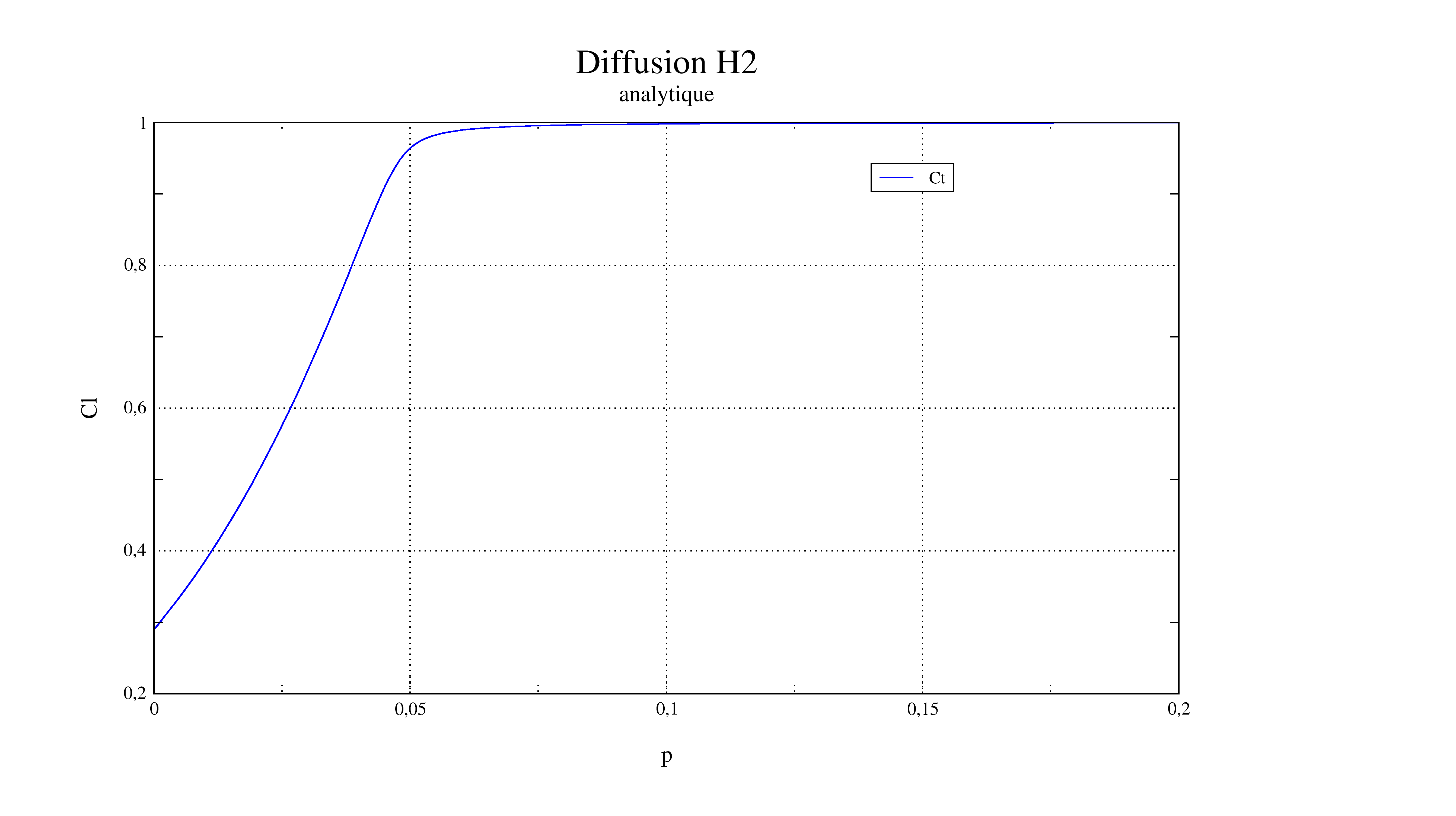
The representation of \({C}_{T}({\varepsilon }_{\mathrm{eq}}^{p})\) and \({C}_{L}({\varepsilon }_{\mathrm{eq}}^{p})\) obtained analytically and numerically in [1] is:

2.2. Benchmark results

2.3. Uncertainty about the solution

Uncertainty less than \(\text{1 \%}\).

2.4. Bibliographical references

1. « Hydrogen transport near a blunting crack tip » A.H.M. Krom, R.W.J.Koers, A.Bakker in « Journal of the Mechanics and Physics of Solids » 45 (1999) 971-992