3. Modeling A#
3.1. Characteristics of modeling#
The mesh is made with elements of the TRIA3 type. The calculation is done in linear elasticity with the operator STAT_NON_LINE.
Spatial error maps for the Zhu-Zienkiewicz indicator version 1 (ERZ1_ELEM) and for the pure residue indicator (ERME_ELGA) are calculated. Beforehand you must have calculated the constraint field at the nodes (SIGM_ELNO) and, to post-process the error map (via GIBI), you must transform it from a CHAM_ELEM per element to a CHAM_ELEM at the nodes per element. The value of the arrow (POST_RELEVE_T) and of the potential deformation energy (POST_ELEM) is also determined.
Everything is placed in a PYTHON loop allowing the implementation of a uniform refinement procedure in nb_calc=4 levels (via MACR_ADAP_MAIL option UNIFORME =” RAFFINEMENT “).
We can thus observe the convergence of the arrow and energy values, the increase in their relative errors with respect to the errors provided by the indicators (themselves in relative terms and over the whole structure), the variations in the efficiency indices of the indicators and their good verification of the saturation hypothesis.
In order to illustrate « good practice » advice for the quality of studies, on the aspects of mesh geometry, mesh itself and the type of finite elements, we use the adhoc options of LIRE_MAILLAGE, MACR_ADAP_MAIL and MACR_INFO_MAIL.
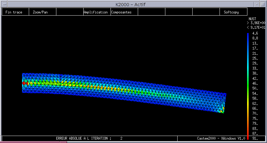
Figure 3.1-a: Isovalues of the residual error (absolute component ERREST) on the initial mesh.
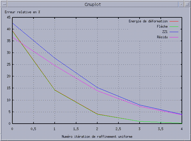
Figure 3.1-b: Decreases in the relative errors of the deformation energy and the deflection compared to those of the relative total component of the indicators.
3.2. Characteristics of the mesh#
Initially: 61 TRIA3, 15 SEG2, 48 knots
After uniform refinement: 244 TRIA3, 30 SEG2, 156 knots
After two uniform refinements: 976 TRIA3, 60 SEG2, 555 knots
After three uniform refinements: 3904 TRIA3, 120 SEG2, 2085 knots
After four uniform refinements: 15616 TRIA3, 240 SEG2, 8073 knots
3.3. Tested sizes and results#
We test the values of the relative errors in deflection and in potential deformation energy with respect to the reference solutions (cf. [§2.2]). And this, on the initial mesh and after four uniform refinements. Since the tests must be multi-platform, the relative tolerance, which is on initial errors set at 10—6%, is deliberately relaxed on errors after four refinements: 10— 4%.
These tests are carried out on variables PYTHON (via TEST_FONCTION) previously inserted into functions ASTER (via FORMULE).
Identification |
Values Code_Aster |
Values of reference |
Tolerance |
Relative variance |
||
(in%) » |
Variable ASTER |
Variable PYTHON |
||||
Ep (0) |
39.406851% |
same |
10— 6% |
—1.26 10—12 ~ 0% |
|
eren0 |
Ep (4) |
0.274116% |
same |
10— 4% |
1.5 10—12 |
||
~ 0% « |
|
eren4 |
||||
Arrow (0) |
39.244715% |
same |
10— 6% |
1.09 10—13 |
||
~ 0% « |
|
erfl0 |
||||
Arrow (4) |
0.270896% |
same |
10— 4% |
—2.25 10—13 ~ 0% |
|
erfl4 |
3.4. What to remember from this part of the TP…#
MACR_INFO_MAIL is therefore complementary to LIRE_MAILLAGE (VERI_MAIL and INFO) and () and**** POST_ELEM. Their combined « efforts » can therefore make it possible to: **
check the correspondence of the mesh with the initial geometry (in mass, dimension, area and volume),
list GROUP_MA and GROUP_NO, which are essential for a good modeling of boundary conditions,
diagnose possible problems (symmetrization or connectedness, draft elements still present in the model, consideration of boundary conditions on surfaces or lines of poor dimensions, interpenetration of elements),
evaluate the quality of the mesh from a strictly finite element point of view.
As close as possible to 1
For example, an empirical criterion could be:
at least 50% of the finite elements with a quality criterion below 1.5,
at least 90%, below 2.
The « thermo-mechanical operators/ MACR_ADAP_MAIL OPTION “UNIFORME” » sequence makes it possible to converge a mesh cleanly, automatically and easily. However, you must be careful about the number of degrees of freedom generated, which can quickly become prohibitive!