4. B modeling#
4.1. Characteristics of modeling#
It is a hardware test. To do this, we use the SIMU_POINT_MAT command, which allows calculation on a single element, with a single integration point.
The loading path between point \(A\) and point \(B\) is discretized in 1 step of time. But we use a fairly recent feature that allows the time step to be re-divided if an additional criterion is not verified at convergence. Here, it is proposed to verify that at each convergence, the cumulative plastic deformation increment does not exceed 0.2 10-2. As soon as this criterion is not met, then the code automatically re-cuts the time step and starts again until this criterion is met.
As an indication, 25 calculations are thus carried out between point \(A\) and point \(B\), this time discretization is therefore qualified as fine, compared to that used in modeling A.
We recall that the point \(A\) corresponds to the instant \(t=\mathrm{1s}\) and the point \(B\) corresponds to the instant \(t=\mathrm{2s}\).
4.2. Tested sizes and results#
Identification |
Instants |
Reference |
\(\text{\%}\) difference |
\({\varepsilon }_{\mathrm{xx}}\) |
|
1.4830 10—2 |
—0.002 |
\({\varepsilon }_{\mathrm{xy}}\) |
|
1.3601 10—2 |
0.003 |
\({\varepsilon }_{\mathrm{xx}}\) |
|
3.5265 10—2 |
0.39 |
\({\varepsilon }_{\mathrm{xy}}\) |
|
2.0471 10—2 |
1.1 |
We can see graphically on the the difference in deformation \({\varepsilon }_{\mathrm{xy}}\) between a fine temporal discretization (modeling B) and a coarse temporal discretization (5 time steps, modeling A). This difference only exists for the non-radial part of the load (beyond point \(A\)). We can clearly see that for modeling B, the time step becomes quite small when approaching point \(B\), just before the moment \(t=\mathrm{2s}\).
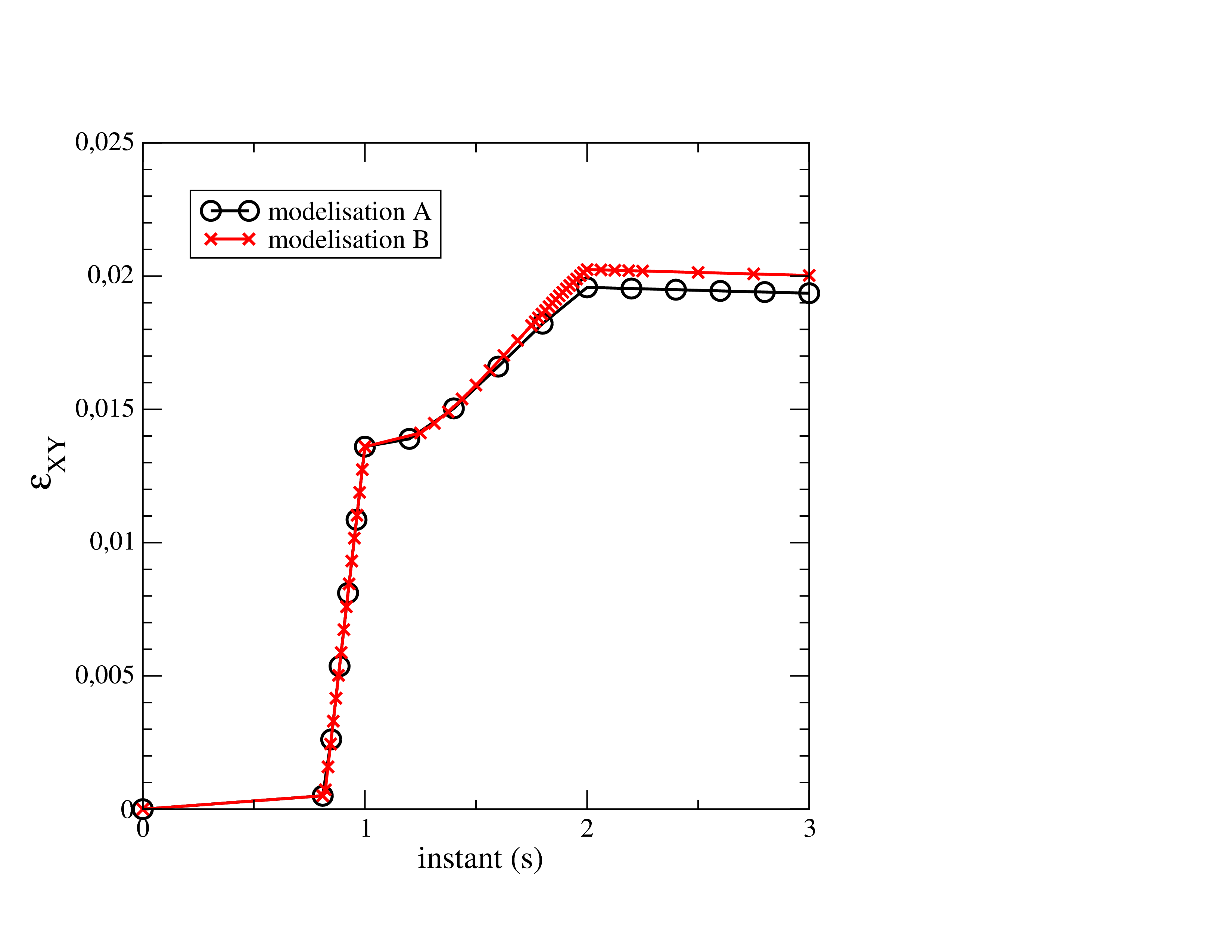
Figure 4.2-1: comparison between different time discretizations