2. Modeling#
2.1. Characteristics of the mesh#
The mesh consists of 5 knots, 4 SEG2 stitches and 3 POI1 stitches.
2.2. Characteristics of modeling#
Regarding the mesh, the springs connecting mleft and mright to the support are modeled by discrete elements (DIS_T) carried on the linear segments (SEG2). The three levels (supports) are modelled by discrete elements (DIS_TR), Three masses are modelled by discrete elements DIS_Tportés by the elements POI1. It is important to emphasize that, for the construction of modal bases, it is necessary to model the relationships between the masses by means of a discrete (DIS_T) carried by a linear segment (SEG2) whose stiffness is very low.
2.3. Modeling parameters#
2.3.1. Modeling A#
Modeling A corresponds to the case where the masses collide with each other. The frontal shock relationship is modelled via RELATION = “DIS_CHOC” and therefore characterized by a normal stiffness of stiffness (shock modeling with penalty) as well as damping linked to the speed of relative movement between masses:
Shock between mleft and mcenter: normal stiffness \({k}_{n}\) = 1.0E+7 (N/m)
Shock between mright and mcenter: normal stiffness \({k}_{n}\) = 3.0E+6 (N/m)
The physical distance between masses is 0.1m, corresponding to the distance between masses in the mesh. So the value of the JEUest keyword is zero.
The value of the tangential shock absorption (unit N m/s in USI) is automatically optimized so as to minimize the residual oscillations in adhesion according to the formula:
\({c}_{i}=2\sqrt{({k}_{n}+{k}_{i}){m}_{i}}-2{\mathrm{\xi }}_{i}\sqrt{{k}_{i}{m}_{i}}\)
where i is the index of the predominant mode in the structure’s response.
2.3.2. B modeling#
Modeling B corresponds to the case where the masses are linked together by means of a device representing linear buckling. The buckling relationship is modelled via RELATION = “FLAMBAGE” and therefore characterized by the following parameters:
Settings |
Keywords |
Relationship between mleft and mcenter |
Relationship between mright and mcenter |
|
Limit normal force that causes structure buckling |
FNOR_CRIT |
0.50 (N) |
0.50 (N) |
0.50 (N) |
Limit normal force after buckling that causes residual deformation of the structure. |
|
0.25 (N) |
0.25 (N) |
|
Normal stiffness value before buckling |
RIGI_NOR |
1.00 (N/m) |
5.00 (N/m) |
5.00 (N/m) |
Value of normal stiffness after buckling. |
|
0.0 (N/m) |
0.0 (N/m) |
Table 2.3.2-1
2.3.3. C modeling#
Modeling C corresponds to the case where the masses are linked together by means of an anti-seismic device. The relationship is modelled via RELATION = “ANTI_SISM”. It makes it possible to calculate the non-linear force represented by the anti-seismic device according to the formula:
- math:
{F} _ {D} = {K} = {K} _ {2} x+frac {({K} _ {2}) x} {sqrt {1+ {({K} _ {K} _ {1} _ {1} x/ {1} x/ {1} x/ {P} _ {y})}}} ^ {2}}} +Cmathit {sign} (dot {x}) {) {lele ft|dot {x}frac {x} {x} {{x} _ {mathit {max}}}right|} ^ {mathrm {alpha}}}
and is therefore characterized for this test case by the following parameters:
Keywords |
Notation in the formula |
Values |
RIGI_K1 |
|
6.0E+06 (N/m) |
RIGI_K2 |
|
0.53E+06 (N/m) |
SEUIL_FX |
|
|
C |
\(C\) |
0.07E+05 (Nm/s) |
PUIS_ALPHA |
|
0.2 (-) |
DX_MAX |
|
0.03 (m) |
Table 2.3.3-1
2.3.4. D modeling#
Modeling D corresponds to the case where the masses are linked together by means of a device representing non-linear viscoelastic behavior. The relationship is modelled via RELATION = “DIS_VISC” with a diagram of the device as follows:
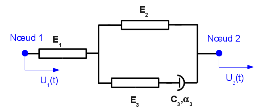
Figure 2.3.4-1
Keywords |
Values |
K1 |
120.00 (N/m) |
K2 |
10.00 (N/m) |
K3 |
60.00 (N/m) |
C |
1.70 (N s/m) |
PUIS_ALPHA |
0.5 (-) |
Table 2.3.4-1
2.3.5. E modeling#
Modeling E corresponds to the case where the masses are linked together by means of a device representing a non-linear behavior defined by a displacement-force function. The relationship is modelled via RELATION = “DIS_ECRO_TRAC”. The function defining the non-linear relationship between mleft and mcenter is provided with the following formula:
\({Y}_{1}(p)={S}_{Y}+\frac{{K}_{p}p}{\sqrt[\mathrm{\rho }]{1+{(\frac{{K}_{p}p}{{S}_{U}-{S}_{Y}})}^{\mathrm{\rho }}}}\)
where:
\({S}_{Y}=200(N)\)
\({S}_{U}=450(N)\)
\({K}_{p}=400(N/m)\)
\(\mathrm{\rho }=1.50\)
value of \(p\) ranging from 0 to 0.2 m with a step of 0.01 m.
The function defining the non-linear relationship between mright and mcenter is defined by the following function:
\({Y}_{2}(p)=0.5{Y}_{1}(p)\)
2.3.6. F modeling#
The F modeling corresponds to the case where a force-displacement relationship on the degree of freedom DX of the mcenter carried node is modeled via RELATION = “RELA_EFFO_DEPL”. The nonlinear function is defined using operator DEFI_FONCTION as follows:
FX_REL = DEFI_FONCTION (NOM_RESU = “FORC”,
NOM_PARA = “DX”,
PROL_GAUCHE =” LINEAIRE “,
PROL_DROITE =” LINEAIRE “,
VALE = (0., 0. ,
1., -1.E5))
2.3.7. G modeling#
The F modeling corresponds to the case where a force-speed relationship on the degree of freedom DX of the mcenter carried node is modeled via RELATION = “RELA_EFFO_VITE”. The nonlinear function is defined using operator DEFI_FONCTION as follows:
FV_REL = DEFI_FONCTION (NOM_RESU = “FORC”,
NOM_PARA = “DX”,
PROL_GAUCHE =” LINEAIRE “,
PROL_DROITE =” LINEAIRE “,
VALE = (0., 0. ,
1., -1.E5))