1. Reference issues#
1.1. Geometry#
Geometry is a compound of 2 segments with 2 nodes. The initial length of segment \(\mathrm{Pt}1-\mathrm{Pt}2\) is \(0.1\mathrm{m}\).

1.2. A, B, C models#
Segment \(\mathrm{Pt}3-\mathrm{Pt}1\) is modeled by a discrete K_T_D_L with ELAS behavior.
Segment \(\mathrm{Pt}1-\mathrm{Pt}2\) is modeled by a discrete K_T_D_L with the CHOC_ENDO behavior.
A mass is assigned to \(\mathrm{Pt}1\).
1.2.1. Common material properties, A, B and C models#
The mass is \(15\mathrm{kg}\). The spring between \(\mathrm{Pt}3-\mathrm{Pt}1\) has a stiffness of \(500\mathrm{N}/\mathrm{m}\) in the x, y, and z directions.
1.2.2. Material properties, modeling A#
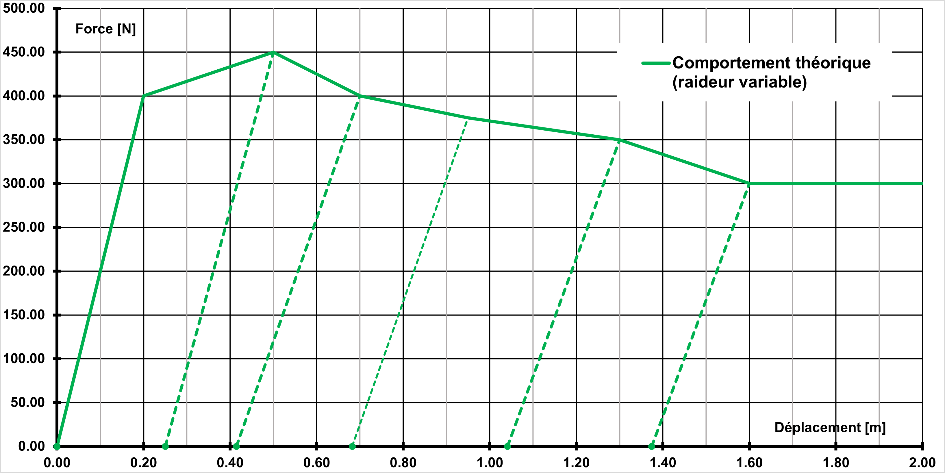
The table above gives the characteristics of the material DIS_CHOC_ENDO, assigned to the discrete \(\mathrm{Pt}1-\mathrm{Pt}2\), for the modeling \(A\).
The stiffness under discharge is constant, the damping is zero.
Ux [m] |
Strength [N] |
Stiffness [N/m] |
Damping [N.s/m] |
0.00 |
0.0 |
2000.0 |
0.0 |
0.20 |
400.0 |
2000.0 |
0.0 |
0.50 |
450.0 |
2000.0 |
0.0 |
0.70 |
400.0 |
2000.0 |
0.0 |
0.95 |
375.0 |
2000.0 |
0.0 |
1.30 |
350.0 |
2000.0 |
0.0 |
1.60 |
300.0 |
2000.0 |
0.0 |
20.0 |
300.0 |
2000.0 |
0.0 |
The figure below shows the behavior corresponding to the data.

The following commands are used to define the material:
ldepla= nu.Array ([0.0, 2.0, 5.0, 7.0, 9.50, 13.0, 16.0, 20.0,]) /10.0
lforce= nu.Array ([0.0, 4.0, 4.5, 4.0, 3.75, 3.50, 3.0, 3.0,]) * 100.0
# Constant stiffness
lraid= nu.Array ([2.0, 2.0, 2.0, 2.0, 2.0, 2.0, 2.0, 2.0,]) * 1000.0
# Depreciation useless in static but mandatory to give
death = nu.Array ([0.0, 0.0, 0.0, 0.0, 0.0, 0.0, 0.0, 0.0,])
#
fctfx = DEFI_FONCTION (NOM_PARA = “X”, ABSCISSE = ldepla, ORDONNEE = lforce, )) **
fctrd = DEFI_FONCTION (NOM_PARA = “X”, ABSCISSE = lrepla, ORDONNEE = stiff, )) **
ctam = DEFI_FONCTION (NOM_PARA = “X”, ABSCISSE = ldepla, ORDONNEE = lamort, )) **
#
Grilleac = DEFI_MATERIAU (
DIS_CHOC_ENDO = _F (
FX = fctfx, RIGI_NOR = fctrd, AMOR_NOR **** = fctam,
DIST_1 = 0.0, DIST_2 ** = 0.0,
CRIT_AMOR = “INCLUS”,
),
)
1.2.3. Material Properties, ModelingB#
The table above gives the characteristics of the material DIS_CHOC_ENDO, assigned to the discrete \(\mathrm{Pt}1-\mathrm{Pt}2\), for the modeling \(B\).
The discharge stiffness is variable, the damping is zero.
Ux [m] |
Strength [N] |
Stiffness [N/m] |
Damping [N.s/m] |
0.00 |
0.0 |
2000.0 |
0.0 |
0.20 |
400.0 |
2000.0 |
0.0 |
0.50 |
450.0 |
1800.0 |
0.0 |
0.70 |
400.0 |
1400.0 |
0.0 |
0.95 |
375.0 |
1400.0 |
0.0 |
1.30 |
350.0 |
1350.0 |
0.0 |
1.60 |
300.0 |
1330.0 |
0.0 |
20.0 |
300.0 |
1330.0 |
0.0 |
Compared to modeling \(A\), only the definition of stiffness changes.
# Variable stiffness
lraid= nu.Array ([2.0, 2.0, 1.8, 1.4, 1.4, 1.35, 1.33, 1.33,]) * 1000.0
The figure below shows the behavior corresponding to the data.
1.2.4. Material properties, C modeling#
The table above gives the characteristics of the material DIS_CHOC_ENDO, assigned to the discrete \(\mathrm{Pt}1-\mathrm{Pt}2\), for the modeling \(C\).
The stiffness under discharge is variable, the damping is variable.
Ux [m] |
Strength [N] |
Stiffness [N/m] |
Damping [N.s/m] |
0.00 |
0.0 |
2000.0 |
2.0 |
0.20 |
400.0 |
2000.0 |
2.0 |
0.50 |
450.0 |
1800.0 |
2.0 |
0.70 |
400.0 |
1400.0 |
1.6 |
0.95 |
375.0 |
1400.0 |
1.6 |
1.30 |
350.0 |
1350.0 |
1.4 |
1.60 |
300.0 |
1330.0 |
1.2 |
20.0 |
300.0 |
1330.0 |
1.2 |
Compared to modeling \(B\), only the definition of depreciation changes.
# Depreciation
lamor= nu.Array ([2.0, 2.0, 2.0, 1.6, 1.6, 1.4, 1.2, 1.2,])
In the material definition CRIT_AMOR = “INCLUS”.