2. Benchmark solution

2.1. Calculation method

You have to solve: \(\rho \mathrm{Cp}\frac{\mathrm{dT}(x,t)}{\mathrm{dt}}=\lambda (t)\frac{\mathrm{dT}(x,t)}{\mathrm{dx}}\) with the initial condition \(T(x\mathrm{,0})=100\) and the boundary conditions: \(-\lambda (t){\frac{\partial T}{\partial x}\mid }_{x=0}=-1\) and \(T(L,t)=100\)

We solve this differential equation with an iterative Crank-Nicholson scheme [1] under scilab.

2.2. Reference quantities and results

The temperature is observed at edge \(x=0\) and in the middle of wall \(x=\frac{L}{2}\). When the conductivity increases between 50 and 55 seconds, the temperature in the medium decreases more rapidly. The waste heat spreads to the edges where warming is observed. This phenomenon is also observed during the drying calculation when the diffusion coefficient depends on the temperature. We then see a re-wetting of the edge.

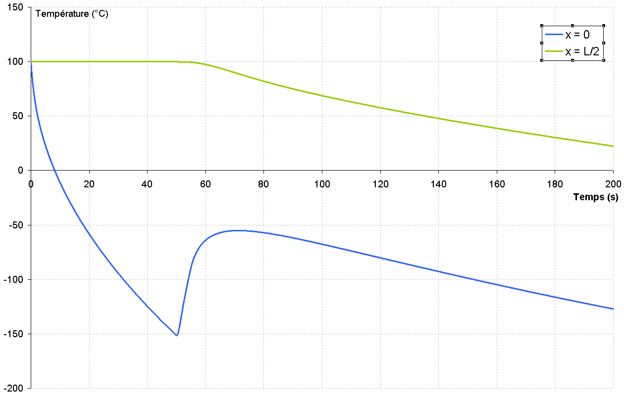
For the reference of the test case, the temperature values in \(x=0\) and \(x=\frac{L}{2}\) are recorded at different times corresponding to the appearance of the temperature jump at the peak and at the end of the calculation.

	50s	51s	72s	200s
x=0	0.0000	0.0000	0.0000	0.0000	0.0000
x=L/2	0.0000	Untested	0.0000	0.0000	0.0000

2.3. Uncertainty about the solution

The resolution method requires steps in time and space that are small enough to properly capture the temperature peak. Here we used \(\mathrm{dx}=\mathrm{0,05}m\) and \(\mathrm{dt}=\mathrm{0,01}s\).

2.4. Bibliographical references

1. 10. Crank, The mathematics of diffusion, Oxford University Press, second edition 1975.