3. Modeling A: FEM 3D#
3.1. Workflow of the TP#
3.1.1. Meshing#
The quadratic mesh of the structure is provided in format MED: forma07a.mmed. Taking into account some symmetries of the problem, only a quarter of the structure is represented. We could only represent \(1\mathrm{/}{8}^{\mathit{ème}}\) of the structure. The mesh was generated with the GIBI software, and tori are defined around the crack bottom:
radius of the smallest torus: \(\mathrm{0,12}m\),
radius of the largest torus: \(\mathrm{0,53}m\).
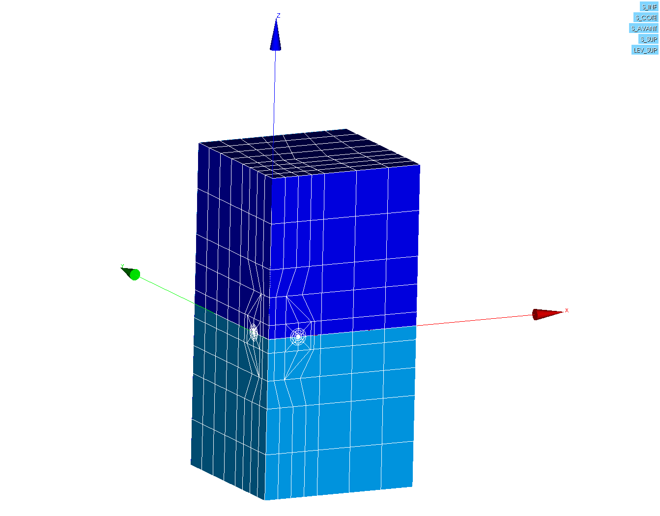
FACE_SUP
FACE_AV Figure 3.1.1-a : Mesh
FACE_INF
FACE_LAT The middle nodes of the edges of the elements touching the bottom of the crack are moved to a quarter of these edges.
3.1.2. Creating the batch file without post-processing the break#
3.1.3. Post-treatment for breakup#
In order to separate calculation and post-processing, you can add a new stage to your case study. |
Define the crack bottom ( DEFI_FOND_FISS **) . Define the crack background in DEFI_FOND_FISSà from the mesh group at the bottom LFFet the lips LEV_INFet LEV_SUP. |
Calculation of G **** and****K****with with**** CALC_G ** (OPTION =( “G”, “K”))). Complete the information on field THETA: * the description of the crack using the keyword FISSURE * the radii of the crown of the theta field (R_INF, R_SUP) (,), to be defined according to the mesh used. Print G values (IMPR_TABLE). |
Calculation of K and G with POST_K1_K2_K3: * fill in the bottom of the crack * fill in the ABSC_CURV_MAXI parameter * print the results in a table (IMPR_TABLE) |
Plot the values of G and K1 from CALC_Get from POST_K1_K2_K3 as a function of the curvilinear abscissa of the crack front (column “ABSC_CURV”) in a spreadsheet. |
3.1.4. To go further: Study of the influence of 3D discretization#
In CALC_G, enter the keyword DISCRETISATION of the keyword factor THETA with the keywords to the value LEGENDRE Compare the values with those obtained previously. As a reminder, when DISCRETISATION is not entered, its value by default is LINEAIRE.
In a second step, add the keyword NB_POINT_FOND =5 to the keyword factor THETAà the discretization LINEAIRE and observe the values of G or K1 along the front. Also compare the calculation times of CALC_G with and without NB_POINT_FOND entered.
3.2. Tested sizes and results#
Identification |
Reference |
% tolerance |
\({K}_{I}\) of POST_K1_K2_K3 |
1.5957 106 |
|