3. Modeling A#
3.1. Characteristics of modeling#
Modeling in shell elements (DKT).
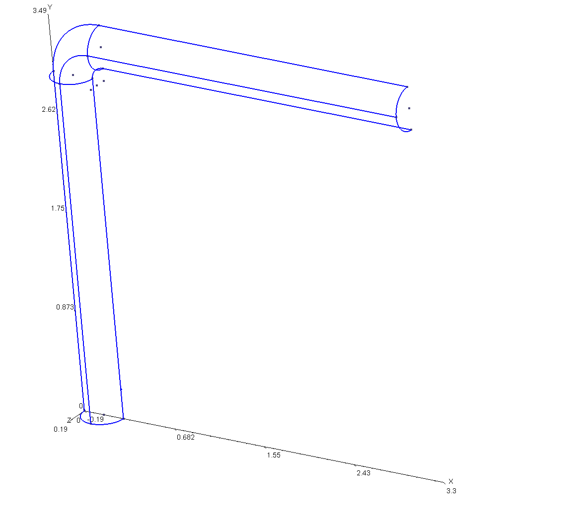
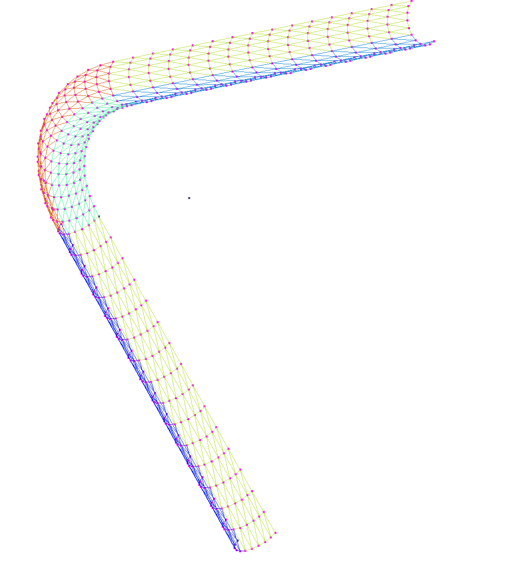
Figure 3.1-a: geometry and mesh of the half cylinder (initial RC)
3.2. Characteristics of the mesh#
The mesh is regenerated at each iteration due to the change in the radius of curvature of the geometry. However, the topological characteristics of the mesh are unchanged:
1013 meshes (900 TRIA3, 110 SEG2, 3 POI3)
507 knots.
The mesh groups correspond to:
\(\mathrm{GM30}\) surface of \(\mathrm{TUYAU}\)
\(\mathrm{GM28}\iff\) section B (effort)
\(\mathrm{GM31}\iff\) point \(\mathrm{A1}\) \((-R,\mathrm{0,}0)\)
\(\mathrm{GM27}\iff\) section \(A\) (embedding)
\(\mathrm{GM29}\iff \mathrm{SYMETRIE}\)
3.3. Aster commands#
This paragraph describes the algorithm used in the command file and introduces the Code_Aster commands used.
Initialization of some variables:
Radius of curvature: \(\mathrm{Rc}=0.3\)
Convergence criterion: \(\mathrm{crit}=2.0E+09\) (target Von Mises constraint)
We enter the python loop whose stopping criterion relates to the Von Mises max constraint. As long as the criterion is not met, the following instructions are carried out:
Reconstruction of the mesh:
we redefine \(\mathrm{Rc}\) in the GMSH geometry.geo file
we launch gmsh via python to generate the.msh mesh file
Reading the mesh (PRE_GMSH) and generating the mesh (LIRE_MAILLAGE). We use DEFI_GROUP to rename mesh groups according to correspondence:
# GM31 <=> A1 # GM27 <=> ENCAST # GM29 <=> SYMETRIE
Definition of the finite elements used (AFFE_MODELE). The straight pipes and the elbow are modeled by shell elements (DKT).
Reorienting the normals to the elements: we use MODI_MAILLAGE to orient all the elements in the same way, with a normal facing inwards.
Definition and assignment of the material (DEFI_MATERIAU and AFFE_MATERIAU). The mechanical characteristics are identical throughout the structure.
Python loop for optimizing the radius of curvature
Assigning the characteristics of shell elements (AFFE_CARA_ELEM): thickness, vector V defining the stripping coordinate system (keyword ANGL_REP)
Definition of boundary conditions and loading (AFFE_CHAR_MECA).
The pipe is embedded at its base, on all the nodes located in the Y=0 plane. The pipe has a \(Z=0\) plane of symmetry.
We calculate a distributed force \(\mathrm{FY}\) directed along the \(Y\) axis and applied to the section \(B\), (the distributed force is such that the resultant \(2\pi \mathrm{.}\mathrm{RMOY.}\mathrm{FY}=\mathrm{FTOT}\), \(\mathrm{FTOT}\) being the total force that one wishes to apply). To apply the effort to section B, we’ll use FORCE_ARETE.
Solving the linear elastic problem (MECA_STATIQUE).
Calculation of the stress field by elements at the nodes for each load case (option “SIGM_ELNO”). The constraints are calculated in the local coordinate system defined for each element using the vector \(V\) (previous ANG_REP keyword). Use NIVE_COUCHE to define the level of calculation in the thickness.
Calculation of the field of equivalent constraints by elements at the nodes calculated from the constraint field (option “SIEQ_ELNO”).
Calculation of the fields preceding the nodes (options” SIGM_NOEU “,” SIEQ_NOEU “)
Printing results (IMPR_RESU).
Determination of a table containing the calculations of averages of the field of stresses equivalent to the nodes. (“POST_RELEVE_T”)
Extracting component VMIS from the previous table via python.
Stop test:
If VMIS is greater than CRIT, then repeat with \(\mathrm{Rc}=\mathrm{Rc}+0.2\)
Otherwise we leave the python loop.