3. Modeling A#
3.1. Characteristics of modeling#
It’s axisymmetric modeling.
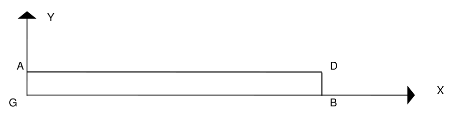
Boundary conditions:
in \(B\) |
|
DY: 0.) |
on \(\mathrm{AG}\) |
|
DX: 0.) |
Loading:
: label: EQ-None
textrm {en} A
Node name:
\(A=\mathrm{N1}\) |
|
|
|
Breakdown: |
100 elements along the radius |
2 elements depending on the thickness |
3.2. Characteristics of the mesh#
Number of knots: 905
Number of meshes and types: 100 QUAD 8, 200 TRIA 6, 200 6, 208 SEG 3
3.3. Tested values#
Location |
Value type |
Reference |
Aster |
% difference |
Point \(A\) |
|
—0.4596 10—3 |
—0.4617 10—3 |
0.46 |
\({e}_{p}(\mathrm{Nm}/\mathrm{rd})\) |
—1.2799 10—2 |
—1.2859 10—2 |
0.47 |
3.4. notes#
The value of the load to be supplied is reduced to a sector of 1 radian. Consequently, the value of the potential energy given on the result file corresponds to the deformation of this sector (to the nearest sign).
Option ENERPOT actually calculates deformation energy:
which is the same as potential energy at the nearest sign:
\({E}_{p}=\frac{1}{2}{U}^{T}KU-{U}^{T}F=-\frac{1}{2}{U}^{T}F=-\frac{1}{2}{U}^{T}KU\) (because \(\mathrm{KU}=F\))