1. Reference problem

1.1. Geometry

Modeling A:

The 2D structure is a single square plate (\(\mathrm{LX}=1\), \(\mathrm{LY}=1\)), with a half-length « breakthrough » crack []. The crack is straight, horizontal, and \(a=\mathrm{0,5}\) in length. The crack is oriented arbitrarily from the right edge to the center.

The edges of the domain are noted trigonometrically:

• \(\mathit{LIG1}\) refers to the bottom edge.

• \(\mathit{LIG2}\) refers to the right edge.

• \(\mathit{LIG3}\) refers to the top edge.

• \(\mathit{LIG4}\) refers to the left edge.

The 4 edges of the domain serve to impose the limit conditions. On the edges not cut by the crack (\(\mathit{LIG1}\), \(\mathit{LIG2}\) , ** \(\mathit{LIG3}\)) Dirichlet boundary conditions are imposed, using the analytical solution while moving (see paragraph [4]).

Note that the right edge (\(\mathit{LIG4}\)) cut by the crack creates a singularity at the intersection. A jump in displacement corresponding to the opening of the crack is observed []. It is difficult to control this edge while moving, since it is necessary to analytically explain the jump condition on the upper lip and on the lower lip of the crack on the edge elements cut by the crack. This difficulty is overcome by imposing Neumann conditions on this side.

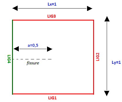
Figure 1.1-1: Domain geometry

B Modeling:

Same geometry as modeling A.

C Modeling:

The crack is tilted at a variable angle such as \(\alpha \epsilon \{{0}^{°}{\mathrm{,30}}^{°}{\mathrm{,60}}^{°}{\mathrm{,90}}^{°}{\mathrm{,120}}^{°}\}\) [].

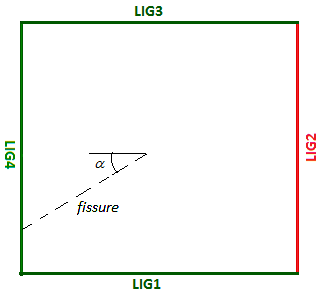
Figure 1.1-2: Inclined crack

Note that the crack has grown longer. The new length is: \(a\mathrm{=}\frac{\mathrm{0,5}}{\mathit{max}\mathrm{\{}∣\mathrm{cos}(\frac{\alpha \mathrm{\times }\pi }{180})∣,∣\mathrm{sin}(\frac{\alpha \mathrm{\times }\pi }{180})∣\mathrm{\}}}\).

1.2. Material properties

Young’s module: \(E={10}^{5}\mathrm{Pa}\)

Poisson’s ratio: \(\nu =0\)

1.3. Boundary conditions and loads

Loading is imposed thanks to mixed boundary conditions.

The uncracked edges are checked when moving, the cracked edge is controlled by force. In addition, the Dirichlet boundary conditions (while moving) fix the structure and prevent the appearance of rigid modes.

In models A and B, the crack only intersects edge \(\mathit{LIG4}\), a Neumann condition is imposed on this edge and a Dirichlet condition on the other 3 edges (see []).

In C modeling, the previous approach is generalized. For an inclination greater than 45°, the crack cuts either the lower edge (\(\mathit{LIG1}\)) or the upper edge (\(\mathit{LIG3}\)). On these two edges, too, a Neumann condition is applied. We therefore impose a Dirichlet condition on the remaining edge (\(\mathit{LIG2}\)) to fix the rigid modes (see []). Since the limit conditions are imposed symmetrically to the horizontal crack (\(\alpha =0\)), the calculations presented will be valid for \(-{135}^{°}<\alpha <{135}^{°}\)

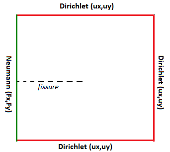
Figure 1.3-1: Mixed boundary conditions for A and B models

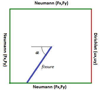
Figure 1.3-2: Mixed boundary conditions for C modeling

The imposed displacement corresponds to the exact analytical solution:

\({U}_{x}=\frac{(1+\nu )}{E}\sqrt{\frac{r}{2\pi }}{K}_{I}\mathrm{cos}(\frac{\theta }{2})(3-4\nu -\mathrm{cos}\theta )\)

\({U}_{y}=\frac{(1+\nu )}{E}\sqrt{\frac{r}{2\pi }}{K}_{I}\mathrm{sin}(\frac{\theta }{2})(3-4\nu -\mathrm{cos}\theta )\)

This solution depends on the polar coordinates linked to the frame of reference of the crack []. In the literature ([13]), the direction of the crack supports the \(\overrightarrow{X}\) axis. Axis \(\overrightarrow{X}\) is oriented from the bottom of the crack to the outside. \(\overrightarrow{Y}\) is orthogonal to \(\overrightarrow{X}\), such that \((\overrightarrow{X},\overrightarrow{Y})\) forms a direct reference frame.

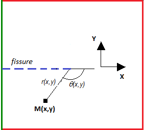
Figure 1.3-3: Local repository of analytical formulas

Consequently, a base change must be made to adapt the valid analytical equations in the crack frame of reference to a given coordinate system. In particular, as the origin of the coordinate system of the cells is chosen in the lower left corner of the domain, the polar coordinates are translated:

\(\theta\) is the polar angle: \(\theta (x,y)=\mathit{arctan2}(y-0.5,x-0.5)\)

\(r\) the radial distance: \(r(x,y)\mathrm{=}\sqrt{{(x\mathrm{-}0.5)}^{2}+{(y\mathrm{-}0.5)}^{2}}\)

The stress tensor for the analytical solution is:

\({\sigma }_{\mathit{xx}}=\frac{{K}_{I}}{\sqrt{2\pi r}}\mathrm{cos}\left(\frac{\theta }{2}\right)\left(1-\mathrm{sin}\left(\frac{\theta }{2}\right)\mathrm{sin}\left(\frac{3\theta }{2}\right)\right)\)

\({\sigma }_{\mathit{yy}}=\frac{{K}_{I}}{\sqrt{2\pi r}}\mathrm{cos}\left(\frac{\theta }{2}\right)\left(1+\mathrm{sin}\left(\frac{\theta }{2}\right)\mathrm{sin}\left(\frac{3\theta }{2}\right)\right)\)

\({\sigma }_{\mathit{xy}}=\frac{{K}_{I}}{\sqrt{2\pi r}}\mathrm{sin}\left(\frac{\theta }{2}\right)\mathrm{cos}\left(\frac{\theta }{2}\right)\mathrm{cos}\left(\frac{3\theta }{2}\right)\)

Then, we project the stress tensor to derive/to establish the force density to be applied on the right edge (\(\mathit{LIG4}\)), from normal « outgoing » \(-\overrightarrow{X}\).

The force to be applied is: \(\overrightarrow{F}\mathrm{=}\underline{\underline{\sigma }}\mathrm{.}\mathrm{-}\overrightarrow{X}\)

It comes: \({F}_{x}=-{\sigma }_{\mathit{xx}}\) and \({F}_{y}=-{\sigma }_{\mathit{xy}}\)

Modeling A:

Relative to the crack reference frame, the « aster » axes are oriented in the same direction. The reference displacement fields \(\mathit{Ux}\) and \(\mathit{Uy}\) are applied to the edges LIG1, LIG2, LIG3:

\({U}_{x}=\frac{E}{2(1+\nu )}\sqrt{\frac{r}{2\pi }}{K}_{I}\mathrm{cos}(\frac{\theta }{2})(3-4\nu -\mathrm{cos}\theta )\)

\({U}_{y}=\frac{E}{2(1+\nu )}\sqrt{\frac{r}{2\pi }}{K}_{I}\mathrm{sin}(\frac{\theta }{2})(3-4\nu -\mathrm{cos}\theta )\)

Likewise, the reference stress tensor is retained. The same force density explained above is therefore applied to edge \(\mathit{LIG4}\).

\({F}_{x}=-{\sigma }_{\mathit{xx}}\) \({F}_{y}=-{\sigma }_{\mathit{xy}}\)

B Modeling:

Same equations as modeling A.

C Modeling:

The crack is tilted at an angle of \(\alpha \epsilon \mathrm{\{}{0}^{°}{\mathrm{,30}}^{°}{\mathrm{,60}}^{°}{\mathrm{,90}}^{°}{\mathrm{,120}}^{°}\mathrm{\}}\).

This rotation impacts the polar angle, the field of displacement, and the stress tensor. These quantities rotate by an angle \(\alpha\), with respect to the fixed coordinate system of the aster code.

\(\theta \to \theta \mathrm{-}\alpha\)

However, this transformation of the polar angle is not valid for all angles, because the definition of the polar angle is not continuous. In the local frame of reference, on either side of the crack, an angular jump of \(2\pi\) is observed: from the lower lip to the upper lip we go from \(-\pi\) to \(\pi\).

Consequently, the rotation of the crack must also propagate this angular discontinuity. All the angles scanned by the crack (gray zone cf. [] and []) during the rotation, undergo an angular jump of \(-2\pi\) or \(2\pi\),

If \(\alpha >0\) (the crack rotates downwards)

• In zone \(\mathrm{-}\pi <\theta <\mathrm{-}\pi +\alpha\) we have: \(\theta \to \theta \mathrm{-}\alpha +2\pi\)

• In zone \(\pi >\theta >\mathrm{-}\pi +\alpha\) we have: \(\theta \to \theta \mathrm{-}\alpha\)

If \(\alpha <0\) (the crack rotates upward)

• In zone \(\pi >\theta >\pi +\alpha\) we have: \(\theta \to \theta \mathrm{-}\alpha \mathrm{-}2\pi\)

• In zone \(\mathrm{-}\pi <\theta <\pi +\alpha\) we have: \(\theta \to \theta \mathrm{-}\alpha\)

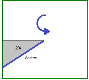
Figure 1.3-4: Angular jump domain (positive)

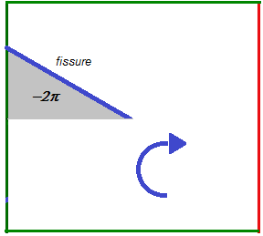
Figure 1.3-5: Angular jump domain (negative)

\(\overrightarrow{U}\to {R}_{\alpha }\overrightarrow{U}\) where \({R}_{\alpha }\) is the angle rotation matrix \(\alpha\) with \({R}_{\alpha }\mathrm{=}\left[\begin{array}{cc}\mathrm{cos}(\alpha )& \mathrm{-}\mathrm{sin}(\alpha )\\ \mathrm{sin}(\alpha )& \mathrm{cos}(\alpha )\end{array}\right]\)

Therefore,

\(\overrightarrow{U}\to \left[\begin{array}{c}\mathrm{cos}(\alpha ){U}_{x}\mathrm{-}\mathrm{sin}(\alpha ){U}_{y}\\ \mathrm{sin}(\alpha ){U}_{x}+\mathrm{cos}(\alpha ){U}_{y}\end{array}\right]\)

The deformation tensor is also impacted by rotation:

\(\underline{\underline{\sigma }}\to {R}_{\alpha }\underline{\underline{\sigma }}{R}_{\mathrm{-}\alpha }\)

\(\underline{\underline{\sigma }}\to \left[\begin{array}{cc}\mathrm{cos}(\alpha )& \mathrm{-}\mathrm{sin}(\alpha )\\ \mathrm{sin}(\alpha )& \mathrm{cos}(\alpha )\end{array}\right]\left[\begin{array}{cc}{\sigma }_{\mathit{xx}}& {\sigma }_{\mathit{xy}}\\ {\sigma }_{\mathit{xy}}& {\sigma }_{\mathit{yy}}\end{array}\right]\left[\begin{array}{cc}\mathrm{cos}(\alpha )& \mathrm{sin}(\alpha )\\ \mathrm{-}\mathrm{sin}(\alpha )& \mathrm{cos}(\alpha )\end{array}\right]\)

\(\underline{\underline{\sigma }}\to \left[\begin{array}{cc}\mathrm{cos}(\alpha )& -\mathrm{sin}(\alpha )\\ \mathrm{sin}(\alpha )& \mathrm{cos}(\alpha )\end{array}\right]\left[\begin{array}{cc}\mathrm{cos}(\alpha ){\sigma }_{\mathit{xx}}-\mathrm{sin}(\alpha ){\sigma }_{\mathit{xy}}& \mathrm{sin}(\alpha ){\sigma }_{\mathit{xx}}+\mathrm{cos}(\alpha ){\sigma }_{\mathit{xy}}\\ \mathrm{cos}(\alpha ){\sigma }_{\mathit{xy}}-\mathrm{sin}(\alpha ){\sigma }_{\mathit{yy}}& \mathrm{sin}(\alpha ){\sigma }_{\mathit{xy}}+\mathrm{cos}(\alpha ){\sigma }_{\mathit{yy}}\end{array}\right]\)

Hence the final writing of the stress tensor:

\(\underline{\underline{\sigma }}\to \left[\begin{array}{cc}\mathrm{cos}{(\alpha )}^{2}{\sigma }_{\mathit{xx}}\mathrm{-}\mathrm{sin}(2\alpha ){\sigma }_{\mathit{xy}}+\mathrm{sin}{(\alpha )}^{2}{\sigma }_{\mathit{yy}}& \mathrm{-}\frac{1}{2}\mathrm{sin}(2\alpha )(\mathrm{-}{\sigma }_{\mathit{xx}}+{\sigma }_{\mathit{yy}})+\mathrm{cos}(2\alpha ){\sigma }_{\mathit{xy}}\\ \mathrm{-}\frac{1}{2}\mathrm{sin}(2\alpha )(\mathrm{-}{\sigma }_{\mathit{xx}}+{\sigma }_{\mathit{yy}})+\mathrm{cos}(2\alpha ){\sigma }_{\mathit{xy}}& \mathrm{sin}{(\alpha )}^{2}{\sigma }_{\mathit{xx}}+\mathrm{sin}(2\alpha ){\sigma }_{\mathit{xy}}+\mathrm{cos}{(\alpha )}^{2}{\sigma }_{\mathit{yy}}\end{array}\right]\)

We check that the rotation maintains the symmetry of the tensor and the trace, \(\mathit{tr}(\underline{\underline{\sigma }})\mathrm{=}{\sigma }_{\mathit{xx}}+{\sigma }_{\mathit{yy}}\)

In the programming of the command file, the horizontal crack is a particular case of an inclined crack: all the equations depend on any \(\alpha\) inclination. To find the A and B models, all you have to do is press \(\alpha \mathrm{=}0°\).

1.4. Benchmark solution

We impose \({K}_{I}\mathrm{=}1\).

In the frame of reference linked to the crack, the analytical equations become:

\({U}_{x}\mathrm{=}\frac{E}{2(1+\nu )}\sqrt{\frac{r}{2\pi }}\mathrm{cos}(\frac{\theta }{2})(3\mathrm{-}4\nu \mathrm{-}\mathrm{cos}\theta )\)

\({U}_{y}\mathrm{=}\frac{E}{2(1+\nu )}\sqrt{\frac{r}{2\pi }}\mathrm{sin}(\frac{\theta }{2})(3\mathrm{-}4\nu \mathrm{-}\mathrm{cos}\theta )\)

By linearity of the equations, the stress tensor is affected by the same proportionality coefficient and becomes:

\({\sigma }_{\mathit{xx}}=\frac{1}{\sqrt{2\pi r}}\mathrm{cos}\left(\frac{\theta }{2}\right)\left(1-\mathrm{sin}\left(\frac{\theta }{2}\right)\mathrm{sin}\left(\frac{3\theta }{2}\right)\right)\)

\({\sigma }_{\mathit{yy}}=\frac{1}{\sqrt{2\pi r}}\mathrm{cos}\left(\frac{\theta }{2}\right)\left(1+\mathrm{sin}\left(\frac{\theta }{2}\right)\mathrm{sin}\left(\frac{3\theta }{2}\right)\right)\)

\({\sigma }_{\mathit{xy}}=\frac{1}{\sqrt{2\pi r}}\mathrm{sin}\left(\frac{\theta }{2}\right)\mathrm{cos}\left(\frac{\theta }{2}\right)\mathrm{cos}\left(\frac{3\theta }{2}\right)\)

By construction, there is no \(\mathit{II}\) mode. In other words, we’re testing \({K}_{\mathit{II}}\mathrm{=}0\).

Modeling A:

This modeling makes it possible to validate the operator POST_ERREUR by comparing the calculated values of the \({L}^{2}\) norm of the displacement and energy of the structure to the analytical values.

1.4.1. Calculation of the L2 norm of displacement

Let \(\Omega\) be the domain occupied by the solid. The \({L}^{2}\) travel standard is defined by:

\({\parallel u\parallel }_{{L}^{2}}^{2}={\int }_{\Omega }{\parallel u\parallel }^{2}\mathit{dS}\mathrm{.}\)

We have:

\({\parallel u\parallel }^{2}={\left(\frac{1+\nu }{E}\right)}^{2}\frac{r}{2\pi }{K}_{I}^{2}{(\kappa -\mathrm{cos}\theta )}^{2},\)

for any \(\Omega\) point. So we have:

\({\parallel u\parallel }_{{L}^{2}}^{2}={\left(\frac{1+\nu }{E}\right)}^{2}\frac{{K}_{I}^{2}}{2\pi }{\int }_{\Omega }r{(\kappa -\mathrm{cos}\theta )}^{2}\mathit{dS}\mathrm{.}\)

Domain \(\Omega\) is represented in Cartesian coordinates by \(\Omega =[-a,a]\times [-a,a]\), where \(a=\mathit{LX}/2=\mathit{LY}/2=1/2\), and can be represented in polar coordinates by:

\(\Omega =\left\{(r,\theta )\in ℝ\times \left[\frac{-\pi }{4},\frac{7\pi }{4}\right],r\le \rho (\theta )\right\},\)

where \(\rho\) is defined by:

\(\rho (\theta )=\{\begin{array}{c}\frac{a}{\mathrm{cos}(\theta )}\text{pour}\theta \in \left[\frac{-\pi }{4},\frac{\pi }{4}\right],\\ \frac{a}{\mathrm{cos}\left(\theta -\frac{\pi }{2}\right)}\text{pour}\theta \in \left[\frac{\pi }{4},\frac{3\pi }{4}\right],\\ \frac{a}{\mathrm{cos}(\theta -\pi )}\text{pour}\theta \in \left[\frac{3\pi }{4},\frac{5\pi }{4}\right],\\ \frac{a}{\mathrm{cos}\left(\theta -\frac{3\pi }{2}\right)}\text{pour}\theta \in \left[\frac{5\pi }{4},\frac{7\pi }{4}\right]\mathrm{.}\end{array}\)

Let’s consider function \(f\mathrm{:}(r,\theta )\to {r}^{n}g(\theta )\). We have:

\(I={\int }_{\Omega }f(r,\theta )\mathit{dS}=\underset{0}{\overset{2\pi }{\int }}\left(\underset{0}{\overset{\rho (\theta )}{\int }}f(r,\theta )r\mathit{dr}\right)d\theta \mathrm{.}\)

So:

\(I=\underset{0}{\overset{2\pi }{\int }}\left(\underset{0}{\overset{\rho (\theta )}{\int }}{r}^{n+1}g(\theta )\mathit{dr}\right)d\theta =\frac{1}{n+2}\underset{0}{\overset{2\pi }{\int }}g(\theta ){\left(\rho (\theta )\right)}^{n+2}d\theta \mathrm{.}\)

We have:

\(J=\underset{0}{\overset{2\pi }{\int }}g(\theta ){\left(\rho (\theta )\right)}^{n+2}d\theta ={J}_{1}+{J}_{2}+{J}_{3}+{J}_{4},\)

with:

\({J}_{1}={a}^{n+2}\underset{\frac{-\pi }{4}}{\overset{\frac{\pi }{4}}{\int }}\frac{g(\theta )}{\mathrm{cos}{(\theta )}^{n+2}}d\theta ,\)

\({J}_{2}={a}^{n+2}\underset{\frac{\pi }{4}}{\overset{3\frac{\pi }{4}}{\int }}\frac{g(\theta )}{\mathrm{cos}{\left(\theta -\frac{\pi }{2}\right)}^{n+2}}d\theta ={a}^{n+2}\underset{\frac{-\pi }{4}}{\overset{\frac{\pi }{4}}{\int }}\frac{g\left(\theta +\frac{\pi }{2}\right)}{\mathrm{cos}{(\theta )}^{n+2}}d\theta ,\)

\({J}_{3}={a}^{n+2}\underset{\frac{3\pi }{4}}{\overset{\frac{5\pi }{4}}{\int }}\frac{g(\theta )}{\mathrm{cos}{(\theta -\pi )}^{n+2}}d\theta ={a}^{n+2}\underset{\frac{-\pi }{4}}{\overset{\frac{\pi }{4}}{\int }}\frac{g(\theta +\pi )}{\mathrm{cos}{(\theta )}^{n+2}}d\theta ,\)

\({J}_{2}={a}^{n+2}\underset{\frac{5\pi }{4}}{\overset{\frac{7\pi }{4}}{\int }}\frac{g(\theta )}{\mathrm{cos}{\left(\theta -\frac{3\pi }{2}\right)}^{n+2}}d\theta ={a}^{n+2}\underset{\frac{-\pi }{4}}{\overset{\frac{\pi }{4}}{\int }}\frac{g\left(\theta +\frac{3\pi }{2}\right)}{\mathrm{cos}{(\theta )}^{n+2}}d\theta ,\)

So we finally have:

\(I=\frac{{a}^{n+2}}{n+2}\underset{\frac{-\pi }{4}}{\overset{\frac{\pi }{4}}{\int }}\frac{1}{\mathrm{cos}{(\theta )}^{n+2}}\left[g(\theta )+g\left(\theta +\frac{\pi }{2}\right)+g(\theta +\pi )+g\left(\theta +\frac{3\pi }{2}\right)\right]d\theta \mathrm{.}\)

We notice that for \(n=1\) and \(g\mathrm{:}\theta \to {(\kappa -\mathrm{cos}(\theta ))}^{2}\)., we have:

\(I={\int }_{\Omega }r{(\kappa -\mathrm{cos}\theta )}^{2}\mathit{dS}\mathrm{.}\)

We also note that:

\({(\kappa -\mathrm{cos}\theta )}^{2}={\kappa }^{2}+\frac{1}{2}-2\mathrm{cos}(\theta )+\frac{1}{2}\mathrm{cos}(2\theta )\mathrm{.}\)

So in this case we have:

\(g(\theta )+g\left(\theta +\frac{\pi }{2}\right)+g(\theta +\pi )+g\left(\theta +\frac{3\pi }{2}\right)=4{\kappa }^{2}+2\mathrm{.}\)

From where:

\({\int }_{\Omega }r{(\kappa -\mathrm{cos}\theta )}^{2}\mathit{dS}=\frac{{a}^{3}}{3}(4{\kappa }^{2}+2)\underset{\frac{-\pi }{4}}{\overset{\frac{\pi }{4}}{\int }}\frac{1}{\mathrm{cos}{(\theta )}^{3}}d\theta \mathrm{.}\)

And finally:

\({\parallel u\parallel }_{{L}^{2}}^{2}={\left(\frac{1+\nu }{E}\right)}^{2}{K}_{I}^{2}{a}^{3}\frac{(2{\kappa }^{2}+1)}{3\pi }\underset{\frac{-\pi }{4}}{\overset{\frac{\pi }{4}}{\int }}\frac{1}{\mathrm{cos}{(\theta )}^{3}}d\theta \mathrm{.}\)

Either:

\({\parallel u\parallel }_{{L}^{2}}=\frac{1+\nu }{E}{K}_{I}{a}^{\frac{3}{2}}\sqrt{\frac{(2{\kappa }^{2}+1)}{3\pi }\underset{\frac{-\pi }{4}}{\overset{\frac{\pi }{4}}{\int }}\frac{1}{\mathrm{cos}{(\theta )}^{3}}d\theta }\approx \mathrm{7,6057690825}\times {10}^{-6}{\text{m}}^{2}\mathrm{.}\)

1.4.2. Calculation of the energy of the structure

The energy of the structure is defined by:

\({E}^{e}=\frac{1}{2}{\int }_{\Omega }\sigma \mathrm{:}\epsilon \mathit{dS}\mathrm{.}\)

Since \(\nu =0\), we have \(\epsilon =\frac{1}{E}\sigma\). From where:

\(\sigma \mathrm{:}\epsilon =\frac{1}{E}\left({\sigma }_{\mathit{xx}}^{2}+{\sigma }_{\mathit{yy}}^{2}+2{\sigma }_{\mathit{xy}}^{2}\right)\mathrm{.}\)

Using the expression for the stress tensor given above and after expansion, we obtain:

\(\sigma \mathrm{:}\epsilon =\frac{{K}_{I}^{2}}{E}\frac{1}{2\pi r}\left(2\mathrm{cos}{\left(\frac{\theta }{2}\right)}^{2}+2\mathrm{cos}{\left(\frac{\theta }{2}\right)}^{2}\mathrm{sin}{\left(\frac{\theta }{2}\right)}^{2}\right)\mathrm{.}\)

We note that:

\(2\mathrm{cos}{\left(\frac{\theta }{2}\right)}^{2}=1+\mathrm{cos}\theta ,\)

\(2\mathrm{cos}{\left(\frac{\theta }{2}\right)}^{2}\mathrm{sin}{\left(\frac{\theta }{2}\right)}^{2}=\frac{1}{2}\mathrm{sin}{(\theta )}^{2}=\frac{1}{4}(1-\mathrm{cos}(2\theta ))\mathrm{.}\)

So we have:

\(\sigma \mathrm{:}\epsilon =\frac{{K}_{I}^{2}}{E}\frac{1}{2\pi r}\left(\frac{5}{4}+\mathrm{cos}(\theta )-\mathrm{cos}(2\theta )\right)\mathrm{.}\)

Either:

\({E}^{e}=\frac{{K}_{I}^{2}}{E}\frac{1}{4\pi }{\int }_{\Omega }\frac{1}{r}\left(\frac{5}{4}+\mathrm{cos}(\theta )-\mathrm{cos}(2\theta )\right)\mathit{dS.}\)

We notice that for \(n=-1\) and \(g\mathrm{:}\theta \to \frac{5}{4}+\mathrm{cos}(\theta )-\mathrm{cos}(2\theta )\)., we have:

\(I=\underset{0}{\overset{\rho (\theta )}{\int }}\frac{1}{r}\left(\frac{5}{4}+\mathrm{cos}(\theta )-\mathrm{cos}(2\theta )\right)d\theta \mathrm{.}\)

In this case, we have:

\(g(\theta )+g\left(\theta +\frac{\pi }{2}\right)+g(\theta +\pi )+g\left(\theta +\frac{3\pi }{2}\right)=5\mathrm{.}\)

From where:

\({\int }_{\Omega }\frac{1}{r}\left(\frac{5}{4}+\mathrm{cos}(\theta )-\mathrm{cos}(2\theta )\right)\mathit{dS}=5a\underset{\frac{-\pi }{4}}{\overset{\frac{\pi }{4}}{\int }}\frac{1}{\mathrm{cos}(\theta )}d\theta =\mathrm{5a}\left(\mathrm{ln}(3)+2\sqrt{2}\right)\mathrm{.}\)

And finally:

\({E}^{e}=\frac{{K}_{I}^{2}}{E}\frac{5a}{4\pi }\left(\mathrm{ln}(3)+2\sqrt{2}\right)\approx \mathrm{3,50687407712}\times {10}^{-6}\text{J}\times {\text{m}}^{-1}\mathrm{.}\)

1.5. Bibliographical references

1. GENIAUT S., MASSIN P.: eXtended Finite Element Method, Code_Aster Reference Manual, [R7.02.12]

2. Rice, J.R. (1968), « A path independent integral and the approximate analysis of strain concentration by notches and cracks, » Journal of Applied Mechanics 35: 379—386

3. Satzi, Belytschko: An extended Finite Element Method with Higher-Order Elements for Curved Cracks

4. LABORDE P., POMMIER J., RENARD Y., Y., SALAUN M., « High-order extended finite element

method for cracked domains », International Journal for Numerical Methods in Engineering, Vl.

64, pp. 354-381, 2005