2. Benchmark solution

2.1. Calculation method

The problem to be solved is:

\({\mathrm{\int }}_{\Omega }\sigma (\frac{\mathrm{\partial }{u}^{\to }}{\mathrm{\partial }x})+\mathrm{\sum }(\frac{\mathrm{\partial }{\nu }^{\to }}{\mathrm{\partial }x})\mathrm{-}\lambda (\frac{\mathrm{\partial }{u}^{\to }}{\mathrm{\partial }x}\mathrm{-}{\nu }^{\to })+{\lambda }^{\to }(\frac{\mathrm{\partial }u}{\mathrm{\partial }x}\mathrm{-}\nu )+r(\frac{\mathrm{\partial }u}{\mathrm{\partial }x}\mathrm{-}\nu )(\frac{\mathrm{\partial }{u}^{\to }}{\mathrm{\partial }x}\mathrm{-}{\nu }^{\to })\mathrm{=}0\)

with \(\forall {u}^{},{\nu }^{},{\lambda }^{}\) cinematically eligible.

We have:

\(\mathrm{\{}\begin{array}{c}\sigma \mathrm{=}E\frac{\mathrm{\partial }u}{\mathrm{\partial }x}\\ \Sigma \mathrm{=}F\frac{\mathrm{\partial }\nu }{\mathrm{\partial }x}\end{array}\)

Let’s note \(\omega\) the second-order form functions and \(\text{N}\) the first-order form functions on linear elements,

At the same time, let’s recall the definitions of SEG2 and SEG3:

SEG2: 2-node segment

number of knots: 2

number of vertex nodes: 2

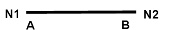
Figure 2.1-a

SEG3: 3-node segment

number of knots: 3

number of vertex nodes: 2

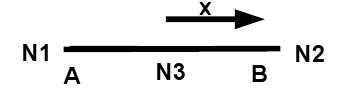
Figure 2.1-b

\({N}_{1}=\frac{1-x}{2}\) and \({N}_{2}=\frac{1+x}{2}\) on the reference element \(x\in \left[-\mathrm{1,}+1\right]\) with \({N}_{1}\) the form function

at the first node.

The shape functions of the segment at the 3 nodes are then:

\({\omega }_{1}=-\frac{x(1-x)}{2}\) \({\omega }_{2}=\frac{x(1+x)}{2}\) and \({\omega }_{3}=1-{x}^{2}\)

By setting \({u}^{}={\nu }^{}=0\) we show that:

\({\int }_{-1}^{+1}{\lambda }^{}(\frac{\partial u}{\partial x}-\nu )\mathrm{dx}=0\) or \(u={\omega }_{1}\mathrm{.}{u}_{1}+{\omega }_{2}\mathrm{.}{u}_{2}+{\omega }_{3}\mathrm{.}{u}_{3}\) with \({u}_{2}=0\) (\(\text{C.L.}\))

Hence \(\frac{\partial u}{\partial x}=(x-\frac{1}{2}){u}_{1}-2x{u}_{3}\) and \(v={N}_{1}\mathrm{.}{\nu }_{1}+{N}_{2}\mathrm{.}{\nu }_{2}\) with \({\nu }_{2}=0\) (\(\text{C.L.}\))

So we have \(\nu =\frac{(1-x)}{2}{\nu }_{1}\) but it should be noted after integration that: \({\nu }_{1}=-{u}_{1}\) (1) \(\forall {u}^{},{\nu }^{},{\lambda }^{}\) kinematically eligible.

Proceeding in the same way and asking: \({\nu }^{}={\lambda }^{}=0\) we find that:

\({u}_{3}=\frac{2(E-r)}{4(E+r)}\mathrm{.}{u}_{1}\approx -\frac{{u}_{1}}{4}\) (2)

Hence the general formula \({S}_{1}={\mathrm{3.a}}^{1}\mathrm{.}\frac{\partial \nu }{\partial x}=-\frac{3}{2}\mathrm{.}{a}^{1}\mathrm{.}{\nu }_{1}\) and after simplification \({S}_{1}=\frac{3}{2}\mathrm{.}{a}^{1}\mathrm{.}{u}_{1}\).

2.2. Reference quantities and results

The fundamental and very general formula for solid is \({S}_{1}=\frac{3}{2}\mathrm{.}{a}^{1}\mathrm{.}{u}_{1}\).

2.3. Uncertainties about the solution

Analytical solution.