5. Appendix#
5.1. Presentation#
We consider the gantry opposite, subject to various loads.

|
We consider the gantry opposite, subject to various loads.
|
Degree 1 hyperstaticity.
Hyperstatic unknown: \(X\)
Charges applied:
moment in \(C\),
vertical loading distributed \(p\) over \({C}_{1}{C}_{2}\),
force \(\mathrm{F1}\), \(\mathrm{F2}\) applied in \({C}_{1}\),
\(\Gamma\) torque applied in \({C}_{1}\)
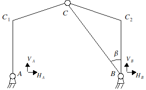
\(\mathrm{tan}(\alpha )=\frac{\mathrm{2a}}{l}=0.4(\Rightarrow {(\mathrm{cos}(\alpha ))}^{-1}=\sqrt{1.16}=1.077033)\)
\(\mathrm{tan}(\beta )=\frac{l}{2(a+h)}=\frac{1}{1.2}\)
\(b=\frac{l}{\mathrm{2cos}(\alpha )};\mathrm{sin}(\alpha )=\frac{a}{b}\)
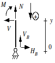
5.2. Isostatic stresses under real load distributed \(p\) on \({C}_{1}C\)#
5.2.1. Isostatic support reactions#
\({H}_{A}+{H}_{B}=0\) \({V}_{A}+{V}_{B}=\frac{\mathrm{pl}}{\mathrm{2cos}(\alpha )}\) \({\mathrm{lV}}_{B}=\frac{{\mathrm{pl}}^{2}}{\mathrm{8cos}(\alpha )}\)
Part \(\mathrm{CB}\) is articulated and loaded only at its ends
\((\begin{array}{}{H}_{B}\\ {V}_{B}\end{array})\wedge \mathrm{BC}=0\iff {H}_{B}=-{V}_{B}\mathrm{tan}(\beta )\)
Hence the isostatic reactions
\({H}_{A}=\frac{\mathrm{pl}}{\mathrm{8cos}(\alpha )}\mathrm{tan}(\beta )\); \({V}_{A}=\frac{3\mathrm{pl}}{\mathrm{8cos}(\alpha )}\); \({H}_{B}=\frac{-\mathrm{pl}}{\mathrm{8cos}(\alpha )}\mathrm{tan}(\beta )\); \({V}_{B}=\frac{\mathrm{pl}}{\mathrm{8cos}(\alpha )}\)
Note:
5.2.2. \(\frac{l\mathrm{tan}(\beta )}{8\mathrm{cos}(\alpha )}=\frac{\mathrm{bl}}{8(a+h)}\)#
5.2.3. Solicitations#
Beam \({\mathrm{AC}}_{1}\)

|
\(\begin{array}{}{N}_{\mathrm{iso}}=\frac{-3\mathrm{pl}}{\mathrm{8cos}(\alpha )}\\ {V}_{\mathrm{iso}}=\frac{\mathrm{pl}}{\mathrm{8cos}(\alpha )}\mathrm{tan}(\beta )\\ {M}_{\mathrm{iso}}=\frac{-\mathrm{pl}}{\mathrm{8cos}(\alpha )}\mathrm{y.tan}(\beta )\end{array}\) |
Beam \({C}_{2}B\)
|
\(\begin{array}{}{N}_{\mathrm{iso}}=\frac{-\mathrm{pl}}{\mathrm{8cos}(\alpha )}\\ {V}_{\mathrm{iso}}=\frac{-\mathrm{pl}}{\mathrm{8cos}(\alpha )}\mathrm{tan}(\beta )\\ {M}_{\mathrm{iso}}=\frac{-\mathrm{pl}}{\mathrm{8cos}(\alpha )}\mathrm{y.tan}(\beta )\end{array}\) |
Beam \({C}_{1}C\)

|
\(\begin{array}{cc}{N}_{\mathrm{iso}}& \text{=}-{H}_{A}\mathrm{cos}(\alpha )-{V}_{A}\mathrm{sin}(\alpha )+\frac{\mathrm{px}}{\mathrm{cos}(\alpha )}\mathrm{sin}(\alpha )\\ & \text{=}-\frac{\mathrm{pl}}{8}(\mathrm{tan}(\beta )+3\mathrm{tan}(\alpha )-8\mathrm{tan}(\alpha )\frac{x}{l})\end{array}\)
|
\({M}_{\mathrm{iso}}=\frac{-\mathrm{pl}}{8(a+h)}(2{s}^{2}(\frac{a+h}{b})-s(\mathrm{2a}+\mathrm{3h})+\mathrm{bh})\) with \(s=\frac{x}{\mathrm{cos}(\alpha )}\in [\mathrm{0,}b]\)
Beam \({\mathrm{CC}}_{2}\)

|
\(\begin{array}{cc}{N}_{\mathrm{iso}}& \text{=}{H}_{B}\mathrm{cos}(\alpha )-{V}_{B}\mathrm{sin}(\alpha )\\ & \text{=}-\frac{\mathrm{pl}}{8}(\mathrm{tan}(\beta )+\mathrm{tan}(\alpha ))\end{array}\)
|
5.2.4. Diagrams#
\((b=\frac{l}{\mathrm{2cos}(\alpha )})\)
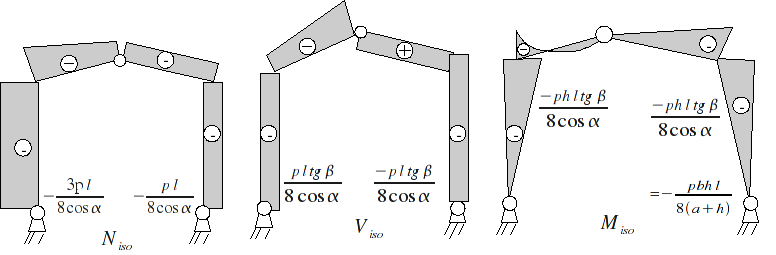
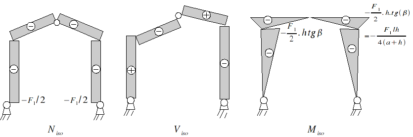
5.3. Concentrated force stresses \({F}_{1}\) (downward)#
5.3.1. Supportive reactions#
\({H}_{A}+{H}_{B}=0;\) \({V}_{A}+{V}_{B}={F}_{1};\) \((\begin{array}{}{H}_{A}\\ {V}_{A}\end{array})\wedge \mathrm{AC}=0=(\begin{array}{}{H}_{B}\\ {V}_{C}\end{array})\wedge \mathrm{BC};\) |

|
From where:
\({H}_{A}=\frac{1}{2}{F}_{1}\mathrm{tan}(\beta )\); \({V}_{A}=\frac{1}{2}{F}_{1}\); \({H}_{B}=\frac{-1}{2}{F}_{1}\mathrm{tan}(\beta )\); \({V}_{B}=\frac{1}{2}{F}_{1}\)
5.3.2. Solicitations#
Beam \({\mathrm{AC}}_{1}\) : |
\({N}_{\mathrm{iso}}=\frac{-1}{2}{F}_{1}\) \({V}_{\mathrm{iso}}=\frac{1}{2}{F}_{1}\mathrm{tan}(\beta )\) \({M}_{\mathrm{iso}}=\frac{-1}{2}{F}_{1}y\mathrm{tan}(\beta )\) |
Beam \({C}_{2}B\) : |
\({N}_{\mathrm{iso}}=\frac{-1}{2}{F}_{1}\) \({V}_{\mathrm{iso}}=\frac{-1}{2}{F}_{1}\mathrm{tan}(\beta )\) \({M}_{\mathrm{iso}}=\frac{-1}{2}{F}_{1}y\mathrm{tan}(\beta )\) |
Beam \({C}_{1}C\) : |
\({N}_{\mathrm{iso}}=\frac{-1}{2}{F}_{1}(\mathrm{tan}(\beta )\mathrm{cos}(\alpha )+\mathrm{sin}(\alpha ))\) \({V}_{\mathrm{iso}}=\frac{1}{2}{F}_{1}(\mathrm{tan}(\beta )\mathrm{sin}(\alpha )-\mathrm{cos}(\alpha ))\) \({M}_{\mathrm{iso}}=\frac{-1}{2}{F}_{1}(y\mathrm{tan}(\beta )-x)\) |
Beam \({\mathrm{CC}}_{2}\) : |
\({N}_{\mathrm{iso}}=\frac{-1}{2}{F}_{1}(\mathrm{tan}(\beta )\mathrm{cos}(\alpha )+\mathrm{sin}(\alpha ))\) \({V}_{\mathrm{iso}}=\frac{1}{2}{F}_{1}(\mathrm{tan}(\beta )\mathrm{sin}(\alpha )-\mathrm{cos}(\alpha ))\) \({M}_{\mathrm{iso}}=\frac{-1}{2}{F}_{1}(y\mathrm{tan}(\beta )-(l-x))\) |
5.3.3. Diagrams (\({F}_{1}\) down)#
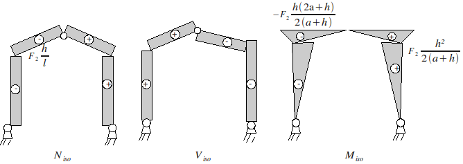
5.4. Solicitations under concentrated force \({F}_{2}\) (to the left)#
5.4.1. Supportive reactions#
\(\begin{array}{}{H}_{A}+{H}_{B}={F}_{2};\\ {V}_{A}+{V}_{B}=0;\\ {\mathrm{lV}}_{B}+{\mathrm{hF}}_{2}=0;\end{array}\)
|

|
From where:
\({H}_{A}={F}_{1}(1-\frac{h}{l}\mathrm{tan}(\beta ))\); \({V}_{A}={F}_{2}\frac{h}{l}\); \({H}_{B}={F}_{1}\frac{h}{l}\mathrm{tan}(\beta )\); \({V}_{B}=-\mathrm{F2}\frac{h}{l}\);
Note:
\(\frac{h}{l}\mathrm{tan}(\beta )=\frac{h}{2(a+h)}\) \((1-\frac{h}{l}\mathrm{tan}(\beta ))=\frac{\mathrm{2a}+h}{2(a+h)}\)
\(\mathrm{tan}(\beta )\mathrm{sin}(\alpha )–\mathrm{cos}(\alpha )=\frac{-\mathrm{hl}}{\mathrm{2b}(a+h)}\), \(\mathrm{tan}(\beta )\mathrm{cos}(\alpha )–\mathrm{sin}(\alpha )=\frac{{l}^{2}–4({a}^{2}+\mathrm{ah})}{\mathrm{4b}(a+h)}\)
5.4.2. Solicitations#
Beam \({\mathrm{AC}}_{1}\): |
\({N}_{\mathrm{iso}}=-{F}_{2}\frac{h}{l}\) \({V}_{\mathrm{iso}}={F}_{2}(1-\frac{h}{l}\mathrm{tan}(\beta ))\) \({M}_{\mathrm{iso}}=-{F}_{2}y(1-\frac{h}{l}\mathrm{tan}(\beta ))\) |
Beam \({C}_{2}B\): |
\({N}_{\mathrm{iso}}={F}_{2}\frac{h}{l}\) \({V}_{\mathrm{iso}}={F}_{2}\frac{h}{l}\mathrm{tan}(\beta )\) \({M}_{\mathrm{iso}}=-{F}_{2}y\frac{h}{l}y\mathrm{tan}(\beta )\) |
Beam \({C}_{1}C\): |
\({N}_{\mathrm{iso}}={F}_{2}((1-\frac{h}{l}\mathrm{tan}(\beta ))\mathrm{cos}(\alpha )–\frac{h}{l}\mathrm{cos}(\alpha ))\) \({V}_{\mathrm{iso}}={F}_{2}((1–\frac{h}{l}\mathrm{tan}(\beta ))–\frac{h}{l}\mathrm{cos}(\alpha ))\) \({M}_{\mathrm{iso}}={F}_{2}(\frac{h}{l}x-(1–\frac{h}{l}\mathrm{tan}(\beta ))y)\) |
Beam \(C{C}_{2}\) : |
\({N}_{\mathrm{iso}}={F}_{2}\frac{h}{l}(\mathrm{tan}(\beta )\mathrm{cos}(\alpha )+\mathrm{sin}(\alpha ))\) \({V}_{\mathrm{iso}}={F}_{2}\frac{h}{l}(\mathrm{tan}(\beta )\mathrm{sin}(\alpha )-\mathrm{cos}(\alpha ))\) \({M}_{\mathrm{iso}}={F}_{2}\frac{h}{l}(y\mathrm{tan}(\beta )-(l-x))\) |
5.4.3. Diagrams#
5.5. Stress under concentrated torque \(\Gamma\) (positive)#
5.5.1. Supportive reactions#
\(\begin{array}{}{H}_{A}+{H}_{B}=0;\\ {V}_{A}+{V}_{B}=0;\\ {\mathrm{lV}}_{B}+\Gamma =0;\end{array}\)
|

|
Where: \({H}_{A}=-\Gamma \mathrm{tan}\frac{\beta }{l}\), \({V}_{A}=\frac{\Gamma }{l}\), \({H}_{B}=\Gamma \mathrm{tan}\frac{\beta }{l}\), \({V}_{A}=\frac{-\Gamma }{l}\)
Note:
\(\frac{\mathrm{tan}(\beta )}{l}=\frac{1}{2(a+h)}\)
5.5.2. Solicitations#
Beam \(A{C}_{1}\): |
\({N}_{\mathrm{iso}}=\frac{-\Gamma }{l}\) \({V}_{\mathrm{iso}}=\frac{-\Gamma \mathrm{tan}(\beta )}{l}\) \({M}_{\mathrm{iso}}=\frac{\Gamma y\mathrm{tan}(\beta )}{l}\) |
Beam \({C}_{2}B\): |
\({N}_{\mathrm{iso}}=\frac{-\Gamma }{l}\) \({V}_{\mathrm{iso}}=\frac{\Gamma \mathrm{tan}(\beta )}{l}\) \({M}_{\mathrm{iso}}=\frac{\Gamma y\mathrm{tan}(\beta )}{l}\) |
Beam \({C}_{1}C\): |
\({N}_{\mathrm{iso}}=\frac{\Gamma }{l}(\mathrm{tan}(\beta )\mathrm{cos}(\alpha )–\mathrm{sin}(\alpha ))\) \({N}_{\mathrm{iso}}=\frac{-\Gamma }{l}(\mathrm{tan}(\beta )\mathrm{sin}(\alpha )+\mathrm{cos}(\alpha ))\) \({N}_{\mathrm{iso}}=\frac{\Gamma }{l}(x+y\mathrm{tan}(\beta )–l)\) |
Beam \(C{C}_{2}\) : |
\({N}_{\mathrm{iso}}=\frac{\Gamma }{l}(\mathrm{tan}(\beta )\mathrm{cos}(\alpha )+\mathrm{sin}(\alpha ))\) \({N}_{\mathrm{iso}}=\frac{\Gamma }{l}(\mathrm{tan}(\beta )\mathrm{sin}(\alpha )-\mathrm{cos}(\alpha ))\) \({N}_{\mathrm{iso}}=\frac{\Gamma }{l}(y\mathrm{tan}(\beta )–(l-x))\) |
5.5.3. Diagrams (\(\Gamma\) positive)#
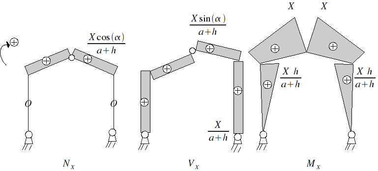
5.6. Solicitations under the \(X\) hyperstatic moment#
5.6.1. Supportive reactions#
\({H}_{A}+{H}_{B}=0;\)
|

|
Hence the reactions: \({H}_{a}=\frac{-X}{a+h}\), \({V}_{A}=0\), \({H}_{B}=\frac{X}{a+h}\), \({V}_{B}=0\)
5.6.2. Solicitations#
Beam \({\mathrm{AC}}_{1}\): |
\({N}_{X}=0\) \({V}_{X}=\frac{-X}{a+h}\) \({M}_{X}=\frac{X}{a+h}y\) |
Beam \({C}_{2}B\): |
\({N}_{X}=0\) \({V}_{X}=\frac{X}{a+h}\) \({M}_{X}=\frac{X}{a+h}y\) |
Beam \({C}_{1}C\): |
\({N}_{X}=\frac{X}{a+h}\mathrm{cos}(\alpha )\) \({V}_{X}=\frac{X}{a+h}\mathrm{sin}(\alpha )\) \({M}_{X}=\frac{X}{a+h}y=\frac{X}{a+h}(h+x\mathrm{tan}(\alpha ))\) |
Beam \({\mathrm{CC}}_{2}\) : |
\({N}_{X}=\frac{X}{a+h}\mathrm{cos}(\alpha )\) \({V}_{X}=\frac{X}{a+h}\mathrm{sin}(\alpha )\) \({M}_{X}=\frac{X}{a+h}y\) |
5.6.3. Diagrams#
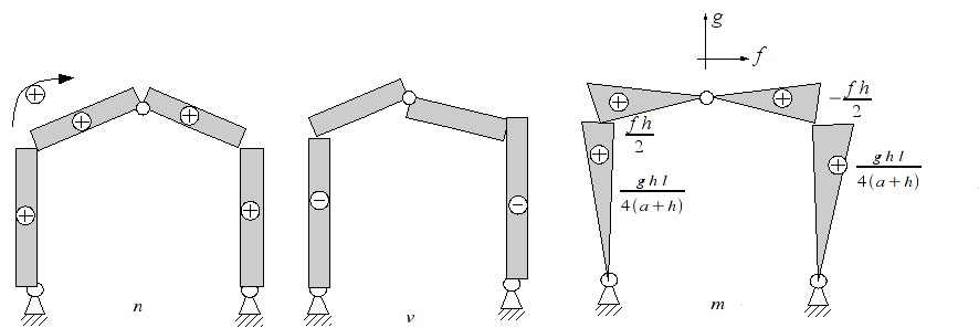
5.7. Requests under fictional one-off loads in \(C\)#
In order to calculate the displacements in \(C\), using the Principle of Virtual Works (\(\mathrm{cf.}\) paragraph \([\S 8]\)), it is necessary to establish the load diagrams under the action of two « fictional » forces \(f\) and \(g\) applied in \(C\).
5.7.1. Supportive reactions#
\({H}_{A}+{H}_{B}=-f;\)
|

|
From where:
\({H}_{A}=\frac{-1}{2}(f+g\mathrm{tan}(\beta ))\), \({V}_{A}=\frac{-1}{2}(g+f\mathrm{cot}(\beta ))\)
\({H}_{B}=\frac{-1}{2}(f-g\mathrm{tan}(\beta ))\), \({V}_{B}=\frac{-1}{2}(g-f\mathrm{cot}(\beta ))\)
5.7.2. Solicitations#
Beam \({\mathrm{AC}}_{1}\) : |
\(n=\frac{1}{2}(g+f\mathrm{cot}(\beta ))\) \(v=\frac{-1}{2}(f+g\mathrm{tan}(\beta ))\) \(m=\frac{1}{2}(f+g\mathrm{tan}(\beta ))\) |
Beam \({C}_{2}B\): |
\(n=\frac{1}{2}(g-f\mathrm{cot}(\beta ))\) \(v=\frac{-1}{2}(f-g\mathrm{tan}(\beta ))\) \(m=\frac{-1}{2}(f-g\mathrm{tan}(\beta ))y\) |
Beam \({C}_{1}C\): |
\(n=\frac{1}{2}(f+g\mathrm{tan}(\beta ))\mathrm{cos}(\alpha )+\frac{1}{2}(g+f\mathrm{cot}(\beta ))\mathrm{sin}(\alpha )\) \(v=\frac{-1}{2}(f+g\mathrm{tan}(\beta ))\mathrm{sin}(\alpha )+\frac{1}{2}(g+f\mathrm{cot}(\beta ))\mathrm{cos}(\alpha )\) \(m=\frac{1}{2}(f+g\mathrm{tan}(\beta ))y-\frac{1}{2}(g+f\mathrm{cot}(\beta ))x\) |
Beam \({\mathrm{CC}}_{2}\) : |
\(n=\frac{-1}{2}(f-g\mathrm{tan}(\beta ))\mathrm{cos}(\alpha )+\frac{1}{2}(g-f\mathrm{cot}(\beta ))\mathrm{sin}(\alpha )\) \(v=\frac{-1}{2}(f-g\mathrm{tan}(\beta ))\mathrm{sin}(\alpha )-\frac{1}{2}(g-f\mathrm{cot}(\beta ))\mathrm{cos}(\alpha )\) \(m=\frac{-1}{2}(f-g\mathrm{tan}(\beta ))y-\frac{1}{2}(g-f\mathrm{cot}(\beta ))(l-x)\) |
5.7.3. Diagrams#
Here are the diagrams of solicitations under the action of the two « fictional » forces \(f\) and \(g\). Here we consider: \(f\ge 0,g\ge \mathrm{fcot}(\beta )\) .
5.8. Determining the \(X\) hyperstatic moment#
We place ourselves in elasticity; we only consider the flexural energy, the beams being slender. The natural state is assumed to be virgin (no prestresses or support movements).
The complementary potential is then:
\(F\ast (X)={\int }_{\mathrm{poteaux}}\frac{{({M}_{\mathrm{iso}}+{M}_{1}X)}^{2}}{{\mathrm{EI}}_{1}}+{\int }_{\mathrm{charpentes}}\frac{{({M}_{\mathrm{iso}}+{M}_{1}X)}^{2}}{{\mathrm{EI}}_{2}}\)
It is stationary at equilibrium, hence:
\(\delta \mathrm{.}X=\left[{\int }_{\mathrm{pot}}\frac{{M}_{1}^{2}}{{\mathrm{EI}}_{1}}+{\int }_{\mathrm{charp}}\frac{{M}_{1}^{2}}{{\mathrm{EI}}_{2}}\right]\mathrm{.}X=-{\int }_{\mathrm{pot}}\frac{{M}_{1}{M}_{\mathrm{iso}}}{{\mathrm{EI}}_{1}}-{\int }_{\mathrm{charp}}\frac{{M}_{1}{M}_{\mathrm{iso}}}{{\mathrm{Ei}}_{2}}=S\)
The flexibility coefficient \(\delta\) is the sum of:
\({\int }_{\mathrm{pot}}\frac{{M}_{1}^{2}}{{\mathrm{EI}}_{1}}=\frac{\mathrm{2h}}{{\mathrm{3EI}}_{1}}{(\frac{h}{a+h})}^{2}\)
\({\int }_{\mathrm{charp}}\frac{{M}_{1}^{2}}{{\mathrm{EI}}_{2}}=\frac{\mathrm{2b}}{{\mathrm{EI}}_{2}}[{(\frac{h}{a+h})}^{2}+\frac{1}{3}{(\frac{a}{a+h})}^{2}+\frac{\mathrm{ah}}{{(a+h)}^{2}}]\)
either:
\(E\mathrm{.}\delta =\frac{2}{{(a+h)}^{2}}[\frac{{h}^{3}}{{\mathrm{3I}}_{1}}+\frac{b({\mathrm{3h}}^{2}+{a}^{2}+\mathrm{3ah})}{{\mathrm{3I}}_{2}}]\)
Digital application:
In the example under consideration:
\({I}_{1}={\mathrm{2I}}_{2}=5.0E-4{m}^{4}\), \(h=\mathrm{2a}=8m\), \(l=20m\), \(b=\frac{l}{2}\sqrt{1.16}\)
From where: \(\gamma =\frac{2}{E{(a+h)}_{1}^{\mathrm{2I}}}\underset{2353.45347{m}^{3}}{\underset{\underbrace{}}{\frac{{h}^{2}}{3}(h+\frac{\mathrm{19b}}{2})}}\)
We study the various loads one after the other to calculate the second members \(S\).
5.8.1. Distributed load \(p\) on \({C}_{1}C\)#
The second member \(S\) due to \(f\) is:
\(-{\int }_{\mathrm{pot}}\frac{{M}_{1}{M}_{\mathrm{iso}}}{{\mathrm{EI}}_{1}}=\frac{\mathrm{3h}}{{\mathrm{3EI}}_{1}}(\frac{h}{a+h})(\frac{\mathrm{pblh}}{8(a+h)})=\frac{2}{E{(a+h)}^{2}{I}_{1}}\frac{{\mathrm{ph}}^{3}\mathrm{bl}}{24}\)
\(-{\int }_{{\mathrm{CC}}_{2}}\frac{{M}_{1}{M}_{\mathrm{iso}}}{{\mathrm{EI}}_{2}}=\frac{{\mathrm{pb}}^{2}\mathrm{hl}}{8(a+h){\mathrm{EI}}_{2}}(\frac{1}{2}\frac{h}{a+h})+(\frac{a}{6}\frac{a}{a+h})=\frac{2}{E{(a+h)}^{2}{I}_{2}}\frac{{\mathrm{phb}}^{\mathrm{2l}}(\mathrm{3h}+a)}{48}\)
\(\begin{array}{}-{\int }_{{C}_{1}C}\frac{{M}_{1}{M}_{\mathrm{iso}}}{{\mathrm{EI}}_{2}}=\frac{1}{{\mathrm{EI}}_{2}}\frac{\mathrm{pl}}{8{(a+h)}^{2}}{\int }_{0}^{b}\left[{\mathrm{2s}}^{2}\frac{a+h}{b}–s(\mathrm{2a}+\mathrm{3h})+\mathrm{bh}\right]\left[h+s\frac{a}{b}\right]\mathrm{ds}\\ =\frac{1}{E{(a+h)}^{2}{I}_{2}}\frac{{\mathrm{plb}}^{2}}{48}({h}^{2}+\mathrm{2ah}+{a}^{2})\end{array}\)
From where:
\(S=\frac{2}{E{(a+h)}^{2}}\frac{\mathrm{plb}}{96}\left[\frac{{\mathrm{4h}}^{3}}{{I}_{1}}+\frac{\mathrm{hb}(\mathrm{3h}+a)}{{I}_{2}}+\frac{b({h}^{2}–\mathrm{2ah}-{a}^{2})}{{I}_{2}}\right]\)
Digital application:
\({I}_{1}=2{I}_{2}\) ; \(h=\mathrm{2a}\) ; \(p=3000{\mathrm{N.m}}^{1}\) (down)
\(S=\frac{2}{E{(a+h)}^{2}{I}_{1}}\underset{43946021.89{\mathrm{N.m}}^{4}}{\underset{\underbrace{}}{\frac{{\mathrm{plbh}}^{2}}{96}\left[\mathrm{4h}+\frac{13}{2}b\right]}}\)
From where:
the moment in \(C\):
\(X=18672994\mathrm{N.m}\)
the reaction in \(A\):
\({H}_{A}=p\frac{\mathrm{bl}}{8(a+h)}-\frac{X}{a+h}=\frac{\frac{\mathrm{pbl}}{8-X}}{a+h}\), \({H}_{A}=5175.37N\)
\({V}_{A}=\frac{\mathrm{3pb}}{4}-0\), \({V}_{A}=24233.24N\)
5.8.2. Point load \({F}_{1}\) in \(C\)#
The second member is obtained using:
\(-{\int }_{\mathrm{pot}}\frac{{M}_{1}{M}_{\mathrm{iso}}}{{\mathrm{EI}}_{1}}=\frac{\mathrm{2h}}{{\mathrm{3EI}}_{1}}(\frac{h}{a+h})(\frac{{F}_{1}\mathrm{lh}}{4(a+h)})=\frac{2}{E{(a+h)}^{2}{I}_{1}}\frac{{F}_{1}{\mathrm{lh}}^{3}}{12}\)
\(-{\int }_{\mathrm{charp}}\frac{{M}_{1}{M}_{\mathrm{iso}}}{{\mathrm{EI}}_{2}}=\frac{\mathrm{2b}}{{\mathrm{EI}}_{2}}\frac{{F}_{1}\mathrm{lh}}{4(a+h)}(\frac{1}{2}(\frac{h}{a+h})+\frac{1}{6}(\frac{a}{a+h}))=\frac{2}{E{(a+h)}^{2}{I}_{2}}\frac{{F}_{1}\mathrm{blh}(\mathrm{3h}+a)}{24}\)
From where:
\(S=\frac{2}{E{(a+h)}^{2}}\frac{{F}_{1}\mathrm{lh}}{24}\left[\frac{{\mathrm{2h}}^{2}}{{I}_{1}}+\frac{b(\mathrm{3h}+a)}{{I}_{2}}\right]\)
Digital application:
\({I}_{1}=2{I}_{2}\) ; \(h=\mathrm{2a}\) ; \({F}_{1}=20000N\) (down)
\(S=\frac{2}{E{(a+h)}^{2}{I}_{1}}\underset{97485127.76{\mathrm{N.m}}^{4}}{\underset{\underbrace{}}{\frac{{F}_{1}{\mathrm{lh}}^{2}}{24}\left[\mathrm{2h}+7b\right]}}\)
From where:
the moment in \(C\):
\(X=41422.161\mathrm{N.m}\)
the reaction in \(A\):
\({H}_{A}=\frac{1}{4}{F}_{1}\frac{l}{a+h}-\frac{X}{a+h}=\frac{\frac{{F}_{1}l}{4-X}}{a+h}\), \({H}_{A}=4881.4866N\)
\({V}_{A}=\frac{1}{2}{F}_{1}-0\), \({V}_{A}=10000.0N\)
5.8.3. Point load \({F}_{2}\) in \({C}_{1}\)#
The second member is obtained using:
\(-{\int }_{{\mathrm{AC}}_{1}}\frac{{M}_{1}{M}_{\mathrm{iso}}}{{\mathrm{EI}}_{1}}=\frac{h}{{\mathrm{3EI}}_{1}}(\frac{h}{a+h})\frac{{F}_{2}h(\mathrm{2a}+h)}{2(a+h)}=\frac{2}{E{(a+h)}^{2}{I}_{1}}\frac{{F}_{2}{h}^{3}(\mathrm{2a}+h)}{12}\)
\(-{\int }_{{C}_{2}B}\frac{{M}_{1}{M}_{\mathrm{iso}}}{{\mathrm{EI}}_{1}}=\frac{h}{{\mathrm{3EI}}_{1}}(\frac{h}{a+h})\frac{(-{F}_{2}{h}^{2})}{2(a+h)}=\frac{2}{E{(a+h)}_{1}^{\mathrm{2I}}}\frac{{F}_{2}{h}^{3}(\mathrm{2a}+h)}{12}\)
\(-{\int }_{{C}_{1}C}\frac{{M}_{1}{M}_{\mathrm{iso}}}{{\mathrm{EI}}_{2}}=\frac{b}{{\mathrm{EI}}_{2}}\frac{{F}_{2}h(\mathrm{2a}+h)}{2(a+h)}\left[\frac{1}{2}(\frac{h}{a+h})+\frac{1}{6}(\frac{a}{a+h})\right]=\frac{2}{E{(a+h)}^{2}{I}_{2}}\frac{{F}_{2}\mathrm{bh}({\mathrm{3h}}^{2}+\mathrm{7ah}+{\mathrm{2a}}^{2})}{24}\)
\(-{\int }_{{\mathrm{CC}}_{2}}\frac{{M}_{1}{M}_{\mathrm{iso}}}{{\mathrm{EI}}_{2}}=\frac{b}{{\mathrm{EI}}_{2}}\frac{-{F}_{2}{h}^{2}}{2(a+h)}\left[\frac{1}{2}(\frac{h}{a+h})+\frac{1}{6}(\frac{a}{a+h})\right]=\frac{2}{E{(a+h)}^{2}{I}_{2}}\frac{-{F}_{2}{\mathrm{bh}}^{2}(\mathrm{3h}+a)}{24}\)
\(S=\frac{2}{E{(a+h)}^{2}}\frac{{F}_{1}\mathrm{lh}}{24}\left[\frac{{\mathrm{2h}}^{2}}{{I}_{1}}+\frac{b(\mathrm{3h}+a)}{{I}_{2}}\right]\)
Digital application:
\({I}_{1}=2{I}_{2}\) ; \(h=\mathrm{2a}\) ****; ** \({F}_{2}=10000N\) (to the left)
\(S=\frac{2}{E{(a+h)}^{2}{I}_{1}}\underset{19497025.55{\mathrm{N.m}}^{4}}{\underset{\underbrace{}}{\frac{{F}_{2}{h}^{2}a}{12}\left[\mathrm{2h}+7b\right]}}\)
From where:
the moment in \(C\):
\(X=8284.4321\mathrm{N.m}\)
the reaction in \(A\):
\({H}_{A}={F}_{2}\frac{\mathrm{2a}+h}{2(a+h)}-\frac{X}{a+h}=\frac{{F}_{2}(a+\frac{h}{2})-X}{a+h}\), \({H}_{A}=5976.297N\)
\({V}_{A}=\frac{{F}_{2}h}{l}\), \({V}_{A}=4000.0N\)
5.8.4. Punctual couple \(\Gamma\) in \({C}_{1}\)#
The second member is obtained using:
\(-{\int }_{\mathrm{pot}}\frac{{M}_{1}{M}_{\mathrm{iso}}}{{\mathrm{EI}}_{1}}=\frac{-\mathrm{2h}}{{\mathrm{3EI}}_{1}}(\frac{h}{a+h})\frac{\Gamma h}{2(a+h)}=\frac{2}{E{(a+h)}^{2}{I}_{1}}\frac{-\Gamma {h}^{3}}{6}\)
\(-{\int }_{{C}_{1}C}\frac{b}{{\mathrm{EI}}_{2}}=\frac{\Gamma (h+\mathrm{2a})}{2(a+h)}\frac{b}{{\mathrm{EI}}_{2}}\left[\frac{1}{2}(\frac{h}{a+h}+\frac{1}{6}(\frac{a}{a+h}))\right]=\frac{2}{E{(a+h)}^{2}{I}_{2}}\frac{\Gamma (h+\mathrm{2a})(\mathrm{3h}+a)b}{24}\)
\(-{\int }_{{\mathrm{CC}}_{2}}\frac{{M}_{1}{M}_{\mathrm{iso}}}{{\mathrm{EI}}_{2}}=\frac{b}{{\mathrm{EI}}_{2}}\frac{-\Gamma h}{2(a+h)}\left[\frac{1}{2}(\frac{h}{a+h})+\frac{1}{6}(\frac{a}{a+h})\right]=\frac{2}{E{(a+h)}^{2}{I}_{2}}\frac{-\Gamma \mathrm{hb}(\mathrm{3h}+a)}{24}\)
From where:
\(S=\frac{2}{E{(a+h)}^{2}}\frac{-\Gamma }{12}\left[\frac{{\mathrm{2h}}^{3}}{{I}_{1}}+\frac{\mathrm{ab}(\mathrm{3h}+a)}{{I}_{2}}\right]\)
Digital application:
\({I}_{1}=2{I}_{2}\) ; \(h=\mathrm{2a}\) ****; ** \(\Gamma =-100000\mathrm{N.m}\) (clockwise)
\(S=\frac{2}{E{(a+h)}^{2}{I}_{1}}\underset{11571281.93{\mathrm{N.m}}^{4}}{\underset{\underbrace{}}{\frac{-\Gamma }{6}\left[{h}^{3}-\mathrm{ab}(\mathrm{3h}+a)\right]}}\)
From where:
the moment in \(C\):
\(X=4916.7243\mathrm{N.m}\)
the reaction in \(A\):
\({H}_{A}=\frac{-\Gamma }{2(a+h)}-\frac{X}{a+h}=\frac{\frac{-\Gamma }{2}-X}{a+h}\), \({H}_{A}=4576.394N\)
\({V}_{A}=\frac{\Gamma }{l}\), \({V}_{A}=5000.0N\)
5.8.5. Recap#
CAS |
Moment in \(C\) |
Reactions in \(A(N)\) |
|
\((\mathrm{N.m})\) |
|
|
|
\(p\) out of \({C}_{1}C\) |
18672.994 |
5175.37 |
24233.240 |
\({F}_{1}\) in \(C\) |
41422.161 |
4881.487 |
10000.000 |
\({F}_{2}\) in \({C}_{1}\) |
8284.432 |
5976.297 |
4000.000 |
\(\Gamma\) in \({C}_{1}\) |
4916.724 |
4576.394 |
5000.000 |
TOTAL |
73296.311 |
22033.31 |
43233.24 |
Note
Reminder: in post \({\mathrm{AC}}_{1}\): normal effort= \(-{V}_{A}\), shear effort= \({H}_{A}\).
5.9. Calculating the displacement in \(C\)#
We also only consider the elastic flexural energy (slender beams). By applying the Principle of Virtual Works on the structure subject to the fictional forces in paragraph \([\S 6]\), working in the movements sought, we calculate the numbers \(w\) and \(d\) depending linearly on \(f\) and \(g\):
\(f{u}_{c}+g{v}_{c}={\int }_{\mathrm{pot}}\frac{m({M}_{\mathrm{iso}}+{\mathrm{XM}}_{1})}{{\mathrm{EI}}_{1}}+{\int }_{\mathrm{charp}}\frac{m({M}_{\mathrm{iso}}+{\mathrm{XM}}_{1})}{{\mathrm{EI}}_{2}}=w+\mathrm{Xd},\forall (f,g)\)
5.9.1. Distributed load \(p\) on \({C}_{1}C\)#
\({\int }_{\mathrm{pot}}\frac{m{M}_{\mathrm{iso}}}{{\mathrm{EI}}_{1}}=\frac{\mathrm{2h}}{{\mathrm{3EI}}_{1}}\frac{\mathrm{ghl}}{4(a+h)}\frac{-\mathrm{pbhl}}{8(a+h)}=\frac{2}{E{(a+h)}^{2}{I}_{1}}\frac{-{\mathrm{gpbh}}^{3}{l}^{2}}{96}\)
\({\int }_{{C}_{1}C}\frac{m{M}_{\mathrm{iso}}}{{\mathrm{EI}}_{2}}=\frac{2}{E{(a+h)}^{2}{I}_{2}}\frac{-{\mathrm{plhb}}^{2}}{384}(\mathrm{2f}(a+h)+\mathrm{gl})(h-a)\)
\({\int }_{{\mathrm{CC}}_{2}}\frac{{M}_{\mathrm{iso}}}{{\mathrm{EI}}_{2}}=\frac{b}{{\mathrm{3EI}}_{2}}\frac{\mathrm{pbhl}}{8(a+h)}(\frac{\mathrm{fh}}{2}-\frac{\mathrm{glh}}{4(a+h)})=\frac{2}{E{(a+h)}^{2}{I}_{2}}\frac{-{\mathrm{pb}}^{2}{\mathrm{lh}}^{2}(\mathrm{gl}-\mathrm{2f}(a+h))}{192}\)
From where:
\(w=\frac{2}{E{(a+h)}^{2}}\frac{-\mathrm{pbhl}}{384}(\frac{{\mathrm{4glh}}^{2}}{{I}_{1}}+\frac{\mathrm{glb}(\mathrm{3h}+a)-\mathrm{efb}{(a+h)}^{2}}{{I}_{2}})\)
Digital application:
\({I}_{1}={\mathrm{2I}}_{2}\); \(h=\mathrm{2a}\); \(p=3000{\mathrm{N.m}}^{-1}\) (down)
\(w=\frac{2}{E{(a+h)}^{2}{I}_{1}}(\mathrm{gl}(\mathrm{2h}+\frac{5}{2}b)-\frac{9}{2}\mathrm{fbh})\underset{-215406.5922{\mathrm{N.m}}^{3}}{\underset{\underbrace{}}{\frac{-{\mathrm{pbh}}^{2}l}{192}}}\)
5.9.2. Point load \({F}_{1}\) in \(C\)#
\({\int }_{\mathrm{pot}}\frac{m{M}_{\mathrm{iso}}}{{\mathrm{EI}}_{1}}=\frac{\mathrm{2h}}{{\mathrm{3EI}}_{1}}\frac{\mathrm{ghl}}{4(a+h)}\frac{-{F}_{1}\mathrm{hl}}{4(a+h)}=\frac{2}{E{(a+h)}^{2}{I}_{1}}\frac{-{F}_{1}{\mathrm{gh}}^{3}{l}^{2}}{48}\)
\({\int }_{\mathrm{charp}}\frac{m{M}_{\mathrm{iso}}}{{\mathrm{EI}}_{2}}=\frac{\mathrm{2b}}{{\mathrm{3EI}}_{2}}\frac{\mathrm{ghl}}{4(a+h)}\frac{-{F}_{1}\mathrm{hl}}{4(a+h)}=\frac{2}{E{(a+h)}^{2}{I}_{2}}\frac{-{F}_{1}{\mathrm{gbh}}^{2}{l}^{2}}{48}\)
Hence (we can see that \(w\) does not depend on \(f\) for this load):
\(w=\frac{2}{E{(a+h)}^{2}}\frac{-{F}_{1}{\mathrm{gh}}^{2}{l}^{2}}{48}(\frac{h}{{I}_{1}}+\frac{b}{{I}_{2}})\)
Digital application:
\({I}_{1}={\mathrm{2I}}_{2}\), \(h=\mathrm{2a}\), \({F}_{1}=20000N\) (down)
\(w=\frac{\mathrm{2g}}{E{(a+h)}^{2}{I}_{1}}\frac{-{F}_{1}{h}^{2}{l}^{2}}{48}\underset{-3155100365.0{\mathrm{N.m}}^{5}}{\underset{\underbrace{}}{(h+\mathrm{2b})}}\)
5.9.3. Point load \({F}_{2}\) in \({C}_{1}\)#
\(\begin{array}{}{\int }_{\mathrm{pot}}\frac{m{M}_{\mathrm{iso}}}{{\mathrm{EI}}_{1}}=\frac{h}{{\mathrm{3EI}}_{1}}\frac{{F}_{2}h}{2(a+h)}\left[-(\mathrm{2a}+h)(\frac{\mathrm{fh}}{2}+\frac{\mathrm{ghl}}{4(a+h)})+h(\frac{-\mathrm{fh}}{2}+\frac{\mathrm{ghl}}{4(a+h)})\right]\\ =\frac{2}{E{(a+h)}^{2}{I}_{1}}\frac{-{F}_{2}{h}^{3}}{24}(\mathrm{agl}+\mathrm{2f}{(a+h)}^{2})\end{array}\)
\({\int }_{\mathrm{charp}}\frac{m{M}_{\mathrm{iso}}}{{\mathrm{EI}}_{2}}=\frac{2}{E{(a+h)}^{2}{I}_{2}}\frac{-{F}_{2}{\mathrm{bh}}^{2}}{24}(\mathrm{agl}+\mathrm{2f}{(a+h)}^{2})\)
From where:
\(w=\frac{2}{E{(a+h)}^{2}}\frac{-{F}_{2}{h}^{2}}{24}(\mathrm{agl}+\mathrm{2f}{(a+h)}^{2})(\frac{h}{{I}_{1}}+\frac{b}{{I}_{2}})\)
Digital application:
\({I}_{1}={\mathrm{2I}}_{2}\), \(h=\mathrm{2a}\), \({F}_{2}=10000N\) (to the left)
\(w=\frac{2}{E{(a+h)}^{2}{I}_{1}}(\mathrm{gl}+\mathrm{9gh})\underset{-3151003.65{\mathrm{N.m}}^{4}}{\underset{\underbrace{}}{\frac{-{F}_{2}{h}^{3}(h+\mathrm{2b})}{48}}}\)
5.9.4. Punctual couple \(\Gamma\) in \({C}_{1}\)#
\(\begin{array}{}{\int }_{\mathrm{pot}}\frac{m{M}_{\mathrm{iso}}}{{\mathrm{EI}}_{1}}=\frac{h}{{\mathrm{3EI}}_{1}}\frac{\Gamma h}{2(a+h)}\left[(\frac{\mathrm{fh}}{2}+\frac{\mathrm{glh}}{4(a+h)})+(\frac{-\mathrm{fh}}{2}+\frac{\mathrm{glh}}{4(a+h)})\right]\\ =\frac{2}{E{(a+h)}^{2}{I}_{1}}\frac{\Gamma {h}^{3}\mathrm{lg}}{24}\end{array}\)
\(\begin{array}{}{\int }_{\mathrm{charp}}\frac{m{M}_{\mathrm{iso}}}{{\mathrm{EI}}_{2}}=\frac{b}{{\mathrm{3EI}}_{2}}\frac{\Gamma h}{2(a+h)}\left[-(\mathrm{2a}+h)(\frac{\mathrm{fh}}{2}+\frac{\mathrm{glh}}{4(a+h)})+h(\frac{-\mathrm{fh}}{2}+\frac{\mathrm{glh}}{4(a+h)})\right]\\ =\frac{-2}{E{(a+h)}^{2}{I}_{2}}\frac{\Gamma \mathrm{bh}}{24}(\mathrm{agl}+\mathrm{2f}{(a+h)}^{2})\end{array}\)
Digital application:
\({I}_{1}={\mathrm{2I}}_{2}\); \(h=\mathrm{2a}\); \(\Gamma =-100000\mathrm{N.m}\)
\(w=\frac{2}{E{(a+h)}^{2}{I}_{1}}\underset{-3151003.65{\mathrm{N.m}}^{4}}{\underset{\underbrace{}}{\frac{\Gamma {h}^{2}}{24}}}(\mathrm{gl}(h-b)-\mathrm{9fhb})\)
5.9.5. Calculation of \(d=\int \frac{m\cdot {M}_{1}}{\mathrm{EI}}\)#
\({\int }_{\mathrm{pot}}\frac{{\mathrm{mM}}_{1}}{{\mathrm{EI}}_{1}}=\frac{\mathrm{2h}}{{\mathrm{3EI}}_{1}}\frac{\mathrm{glh}}{4(a+h)}\frac{h}{a+h}=\frac{2}{E{(a+h)}^{2}{I}^{1}}\frac{{\mathrm{glh}}^{3}}{12}\)
\({\int }_{\mathrm{charp}}\frac{m{M}_{1}}{{\mathrm{EI}}_{2}}=\frac{\mathrm{2b}}{{\mathrm{EI}}_{2}}\left[\frac{1}{2}(\frac{h}{a+h})+\frac{1}{6}(\frac{a}{a+h})\right]\frac{\mathrm{glh}}{4(a+h)}=\frac{2}{E{(a+h)}^{2}{I}_{2}}\frac{\mathrm{glbh}(\mathrm{3h}+a)}{24}\)
From where (we can see that \(d\) does not depend on \(f\)):
\(d=\frac{2}{E{(a+h)}^{2}}\frac{\mathrm{glh}}{24}(\frac{{\mathrm{2h}}^{2}}{{I}_{1}}+\frac{b(\mathrm{3h}+a)}{{I}_{2}})\)
Digital application:
\({I}_{1}=2{I}_{2}\), \(h=\mathrm{2a}\)
\(d=\frac{2}{E{(a+h)}^{2}{I}_{1}}g\frac{{\mathrm{lh}}^{2}}{24}\underset{-4874.2564{\mathrm{N.m}}^{4}}{\underset{\underbrace{}}{(\mathrm{2h}+\mathrm{7b})}}\)
5.9.6. Summary of \({u}_{c}\) and \({v}_{c}\) trips#
\({I}_{1}=5.0E-4{m}^{4}\)
\(E=210000\mathrm{MPA}\)
CAS |
\(X\) |
|
|
press on \({C}_{1}C\) |
18672.994 |
91016960.3 |
—184930109.4 |
\({F}_{1}\) in \(C\) |
41422.161 |
201902233.4 |
—315100365.0 |
\({F}_{2}\) in \({C}_{1}\) |
8284.432 |
40380445.6 |
—63020073.0 |
\(\Gamma\) in \({C}_{1}\) |
4916.724 |
23965373.4 |
14775091.25 |
CAS |
\({w}_{h}\) |
|
|
|
press on \({C}_{1}C\) |
83519999.94 |
0.0110476 |
—0.012422374 |
|
\({F}_{1}\) in \(C\) |
0.00 |
0.00 |
—0.01497330 |
|
\({F}_{2}\) in \({C}_{1}\) |
—226872262.8 |
—0.03000956 |
—0.00299466 |
—0.00299466 |
\(\Gamma\) in \({C}_{1}\) |
206790328.5 |
0.0273532 |
—0.001215646 |
Note:
\(d=\frac{2}{E{(a+h)}^{2}{I}_{1}}g\stackrel{ˉ}{d}\), with: \(\stackrel{ˉ}{d}=4874.2564{m}^{4}\)
\(w=\frac{2}{E{(a+h)}^{2}{I}_{1}}(g{w}_{v}+f{w}_{h})\) see above
\({u}_{c}=\frac{2}{E{(a+h)}^{2}{I}_{1}}{w}_{H}\); \({v}_{c}=\frac{2}{E{(a+h)}^{2}{I}_{1}}({w}_{v}+X\stackrel{ˉ}{d})\)
\(\frac{2}{E{(a+h)}^{2}{I}_{1}}=1.32275132E-10{N}^{-1}{m}^{-4}\)
Comparison Aster- analytical reference (R.)
CAS |
Moment in \(C(\mathrm{N.m})\) |
Reaction \({H}_{A}(N)\) |
Reaction \({V}_{A}(N)\) |
Move \({u}_{c}(m)\) |
Move \({v}_{c}(m)\) |
|
\(P\) out of \({C}_{1}C\) |
R: Aster: |
18672.994 18673.20 |
5175.37 5175.36 |
24233.24 24233.2 |
0.0110476 0.0110472 |
—0.012422374 —0.0124233 |
\({F}_{1}\) in \(C\) |
R: Aster: |
41422.161 41422.40 |
4881.487 4881.47 |
10000.00 10000.0 |
0.00000 0.0000 |
—0.01497330 —0.0 |
\({F}_{2}\) in \({C}_{1}\) |
R: Aster: |
8284.432 8284.34 |
5976.297 5976.31 |
4000.00 4000.0 |
—0.03000956 —0.0300098 |
—0.00299466 —0.00299450 |
\(\Gamma\) in \({C}_{1}\) |
R: Aster: |
4916.724 4916.62 |
4576.394 |
|||
4576.38 » |
5000.00 5000.0 |
0.0273532 0.0273536 |
—0.001215646 —0.00121583 |
Note:
The*Aster* calculation was done by taking very slender elements, so that: \({\mathrm{Sl}}^{2}\ll I\). Thus, the flexural energy is predominant. The values for the Aster calculation are from test case \(\mathrm{VPCS}\) called \(\mathrm{SSLL14}\), with the following data:
\({I}_{1}=5.0E-4{m}^{4}\); \({I}_{2}=2.5E-4{m}^{4}\); \(E=210000\mathrm{MPa}\)
\(h=\mathrm{2a}=8m\); \(l=20m\); \(b=\frac{l}{2}\sqrt{1.16}\)
\(p=3000\mathrm{N.m}\) (down),
\({F}_{1}=20000N\) (down),
\({F}_{2}=10000N\) (to the left),
\(\Gamma =-100000\mathrm{Nm}\) (clockwise)