1. Reference problem#
1.1. Geometry#
Outside diameter |
: |
\(48.E-3m\) |
Thickness |
: |
\(5.E-3m\) |
Elbow radius |
: |
\(0.170m\) |
1.2. Material properties#
Density |
: |
\(7960.{\mathrm{kg.m}}^{-3}\) |
Young’s module |
: |
\(1.9E+11{\mathrm{N.m}}^{-2}\) |
Poisson’s ratio |
: |
\(0.3\) |
Mass concentrated at node 4 |
: |
\(10.\mathrm{kg}\) |
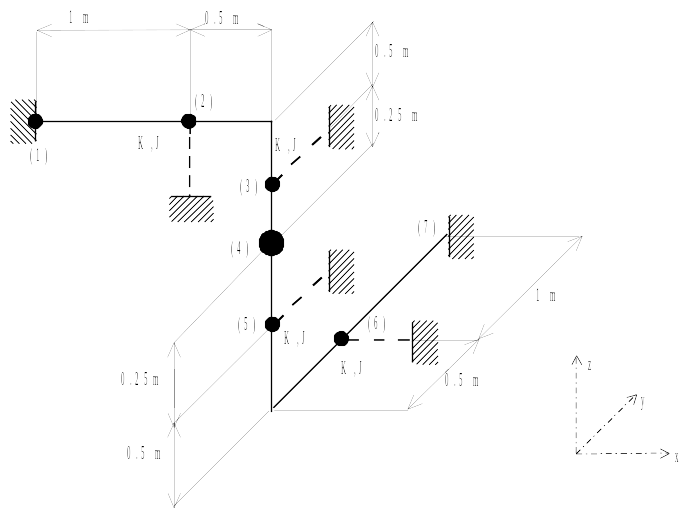
1.3. Boundary conditions and loads#
1.3.1. Boundary conditions#
At node 1: \(\mathrm{dx}=\mathrm{dy}=\mathrm{dz}=0\) (ball joint)
At node 7: \(\mathrm{dx}=\mathrm{dy}=\mathrm{dz}=\mathrm{drx}=\mathrm{dry}=\mathrm{drz}=0\) (embedding)
At node 2, support in direction \(z\)
At node 3, support in direction \(y\)
At node 5, support in direction \(y\)
At node 6, support in the \(x\) direction
The stiffness provided by each of the supports are:
\({K}_{x}={K}_{y}={K}_{z}=80.E+3{\mathrm{N.m}}^{-1}\) \({K}_{\theta x}={K}_{\theta y}={K}_{\theta z}=J=1.2{\mathrm{N.m.deg}}^{-1}\)
1.3.2. Loads#
Calculating static modes
A first calculation makes it possible to validate the calculation of the static modes.
The entire model is subject to a uniform acceleration according to \(x\) with a value of \(100\mathrm{\times }g\) with \(g=9.81{\mathrm{m.s}}^{-2}\)
Spectral response
The pipe line is subjected to an excitation following \(x\), defined by a response spectrum such as:
its value in displacement for frequencies between 1 and 10. \(\mathrm{Hz}\), or \(d=48.E-\mathrm{3m}\)
its speed value for frequencies between 10. and 63. \(\mathrm{Hz}\), or \(v={\mathrm{3.m.s}}^{-1}\)
its acceleration value for frequencies between 63. and 1000. \(\mathrm{Hz}\), or \(\gamma =120\ast g\)
Below is shown the acceleration spectrum, determined from the excitation for reduced damping \(\xi \mathrm{=}0\).
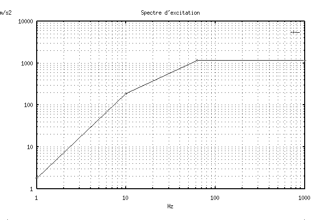
The characteristic values used are:
\(\gamma (1\mathrm{Hz})=\mathrm{1.92m}/{s}^{2}\) \(\gamma (10\mathrm{Hz})=192m/{s}^{2}\) \(\gamma (63\mathit{Hz})\mathrm{=}1000m\mathrm{/}{s}^{2}\)
\(\gamma (1000\mathrm{Hz})=1000m/{s}^{2}\)
1.3.3. Elbow flexibility#
The flexibility coefficient, \({C}_{\mathrm{flex}}\), of the elbows is given by the RCC -M regulation:
\({C}_{\mathrm{flex}}=\frac{1.65}{h}\) with \(h=\frac{\mathrm{ep}\ast {r}_{\mathrm{courb}}}{{r}_{m}^{2}}\)
\(\mathrm{ep}\) |
: |
elbow thickness |
\({r}_{\mathrm{courb}}\) |
: |
elbow radius of curvature |
\({r}_{m}\) |
: |
mean elbow radius |
The stress intensification index, \({I}_{\mathrm{sigm}}\), is given by:
\({I}_{\mathrm{sigm}}=\frac{0.9}{{h}^{0.666}}\)
According to regulation RCC -M, the flexibility coefficient and the stress intensification index are greater than or equal to one. This is not the case in this test case.