3. Modeling A#
3.1. Characteristics of modeling and meshes#
This modeling tests reading dataset 58 from a file in universal format (IDEAS), containing both displacement fields, speed and constraint fields. The expansion is also carried out on the numerical model by exploiting the mixed measurement (displacement, speed and stress).
Digital mesh:
The digital mesh is made with I- DEAS Master Series 5 version. It has 2667 knots and 3328 linear \(\mathrm{3D}\) meshes.
Experimental mesh:
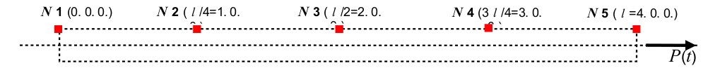
The measurement mesh includes only 5 point elements and 5 nodes positioned as shown in the following figure:
3.2. Characteristics of the measures#
The experimental measurements provided are:
the axial stresses \({\sigma }_{\mathit{xx}}\), in the direction \(x\) at the nodes \(\mathit{N3}\), \(\mathrm{N4}\) and \(\mathrm{N5}\),
the axial displacement at node \(\mathrm{N3}\),
the axial speed at node \(\mathrm{N5}\).
The time sampling is constant: the initial time is \(0s\), the time step is \({10}^{-5}s\), and the number of moments is 1001 (i.e. up to a final time of \(0.01s\)).
The values come from the direct calculation carried out with*Code_Aster*.
3.3. Characteristics of the modal base#
The modes are stored in a concept such as [mode_meca], containing the first three dynamic traction modes. These modes are obtained by blocking the transverse movements (i.e. next \(\mathrm{DY}\) and \(\mathrm{DZ}\)) of the nodes of the neutral fiber and the nodes of the upper line (\(x=0.\) to \(4.\) \(y=0.1\) and \(z=0.\)). Their natural frequencies (\(326.5\mathrm{Hz}\), \(980.0\mathrm{Hz}\) and \(1634.5\mathrm{Hz}\)) are close to the natural traction frequencies calculated analytically (\(324.3\mathrm{Hz}\), \(972.9\mathrm{Hz}\) and \(1621.5\mathrm{Hz}\)).
3.4. Tested sizes and results#
Identification |
Reference |
||
at*t* = 9. 10—4s |
2.686 10—4 |
||
DEPL_X |
At node \(\mathrm{N2}\) |
at*t* = 17. 10—4s |
3.074 10—4 |
\((m)\) |
at*t* = 25. 10—4s |
1.446 10—5 |
|
at*t* = 9. 10—4s |
5.793 10—4 |
||
DEPL_X |
At node \(\mathrm{N4}\) |
at*t* = 17. 10—4s |
9.160 10—4 |
\((m)\) |
at*t* = 25. 10—4s |
3.095 10—4 |
|
at*t* = 9. 10—4s |
6.221 10—1 |
||
VITE_X |
At node \(\mathrm{N2}\) |
at*t* = 17. 10—4s |
—4.683 10—2 |
\((m\mathrm{/}s)\) |
at*t* = 25. 10—4s |
—3.542 10—1 |
|
at*t* = 9. 10—4s |
8.056 10—1 |
||
VITE_X |
At node \(\mathrm{N4}\) |
at*t* = 17. 10—4s |
—3.556 10—1 |
\((m/s)\) |
at*t* = 25. 10—4s |
—8.638 10—1 |
|
at*t* = 9. 10—4s |
—3.633 10+3 |
||
ACCE_X |
At node \(\mathrm{N2}\) |
at*t* = 17. 10—4s |
6.337 10+2 |
\((m/{s}^{2})\) |
at*t* = 25. 10—4s |
3.801 10+3 |
|
at*t* = 9. 10—4s |
8.655 10+2 |
||
ACCE_X |
At node \(\mathrm{N4}\) |
at*t* = 17. 10—4s |
—2.387 10+3 |
\((m/{s}^{2})\) |
at*t* = 25. 10—4s |
—6.355 10+2 |
|
at*t* = 9. 10—4s |
1.957 10—4 |
||
EPXX |
At node \(\mathrm{N2}\) |
at*t* = 17. 10—4s |
3.015 10—4 |
\((m)\) |
at*t* = 25. 10—4s |
5.422 10—5 |
|
at*t* = 9. 10—4s |
1.822 10—4 |
||
EPXX |
At node \(\mathrm{N4}\) |
at*t* = 17. 10—4s |
2.611 10—4 |
\((m)\) |
at*t* = 25. 10—4s |
1.681 10—4 |
|
at*t* = 9. 10—4s |
5.012 10+7 |
||
SIXX |
At node \(\mathrm{N2}\) |
at*t* = 17. 10—4s |
7.717 10+7 |
\((\mathrm{Pa})\) |
at*t* = 25. 10—4s |
1.390 10+7 |
|
at*t* = 9. 10—4s |
4.650 10+7 |
||
SIXX |
At node \(\mathrm{N4}\) |
at*t* = 17. 10—4s |
6.671 10+7 |
\((\mathit{Pa})\) |
at*t* = 25. 10—4s |
4.293 10+7 |
|
\(\mathrm{\sum }_{i}∣{\mathit{depl}}_{x}(\mathit{NRES3})({t}_{i})\mathrm{-}{\mathit{depl}}_{x}(\mathit{N3})({t}_{i})∣\) \((m)\) |
0 |
||
\(\mathrm{\sum }_{i}∣{\mathit{vite}}_{x}(\mathit{NRES5})({t}_{i})\mathrm{-}{\mathit{vite}}_{x}(\mathit{N5})({t}_{i})∣\) \((m/s)\) |
0 |
||
\(\mathrm{\sum }_{i}∣\mathit{SIXX}(\mathit{NRES4})({t}_{i})\mathrm{-}\mathit{SIXX}(\mathit{N4})({t}_{i})∣\) \((\mathrm{Pa})\) |
0 |
||