4. B modeling#
4.1. Characteristics of modeling#
The characteristics used and the mesh are those deduced from the data in paragraph 1. The mesh is the same as for modeling A.
The temporal response has been calculated at point \(N11\) and the corresponding response spectrum has been determined. Since the transfer function is equal to 1 for the case without spatial variability, the temporal response is equal to the input signal. If spatial variability is taken into account, then the response is modified.
In this modeling, we test the various coherence functions available in code_aster (MITA_LUCO, ABRAHAMSON, ABRA_ROCHER, ABRA_SOLMOYEN).
4.2. Characteristics of the mesh#
The characteristics are those of modeling A.
4.3. Tested sizes and results#
4.3.1. Mita & Luco consistency function#
We check that, for \(\alpha =0.0\), the acceleration response is equal to the accelerogram at the input of the calculation (we recall that the transfer function is equal to 1 and that the function is rigid for this case study). The answer \(q(t)\) is determined in “DX” at the point \(N11\) for an excitation \(a(t)\) in “DX”. The error is calculated as the standard deviation of the difference (residual) between the signal and the response. This is done for the case where the transfer function is calculated for all the points (discretization of the accelerogram) and for the case where the user enters FREQ_PAS, FREQ_FIN. In the latter case, DYNA_ISS_VARI interpolates calculated values to determine the temporal response due to the excitation by the accelerogram.
We also add to this case a test of NON_REGRESSION for the maximum positive displacement value in “DX” at the point \(N11\) which corresponds to the center of the foundation.
test type |
reference value |
tolerance (abs.) |
|
ANALYTIQUE |
0.0 |
0.01 |
Likewise, for \(\alpha =0.0\), the oscillator response spectrum (SRO) of the calculated acceleration response must be equal to the SRO of the input accelerogram. So, we test the error, namely the difference between these two SRO. In particular, we compare and evaluate the maximum difference between the two SRO and the standard deviation of the error
test type |
value |
reference value |
tolerance (abs.) |
ANALYTIQUE |
|
0.0 |
0.01 |
ANALYTIQUE |
|
0.0 |
0.001 |
For the case with spatial variability, values \(\alpha =0.7,{V}_{s}=200m/s\) were chosen. We consider a temporal seismic excitation in the “DX” direction given by an accelerogram corresponding to spectrum EUR for a rocky site (cf, red curve in the figure below). There is no reference (analytical) solution for this case. Also, we do a NON_REGRESSION test for the SRO obtained with spatial variability. We’re testing two cases.
FREQ_FIN is equal to the cutoff frequency:
test type |
frequency (Hz) |
reference SRO (g) |
tolerance (%) |
|
NON_REGRESSION |
10.0 |
5.34727E-01 |
2*10-4 |
|
NON_REGRESSION |
30.0 |
2.3855E-01 |
2*10-3 |
2.3855E-01 |
FREQ_FIN is less than the cutoff frequency (\(35Hz\) instead of \(50Hz\)) and we complete by zero:
test type |
frequency (Hz) |
reference SRO (g) |
tolerance (%) |
||
NON_REGRESSION |
10.0 |
5.34727E-01 |
2*10-1 |
NON_REGRESSION |
30.0 |
2.3855E-01 |
2*10-2 |
The response spectra of the accelerogram (SRO_ACCE) and calculated in response to point \(N11\), without spatial variability (SRO_NVAR) and with spatial variability (SRO_VAR), are shown in the figure below:
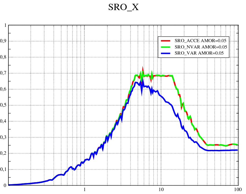
frequency [Hz]
Note: For the test case, the accelerogram EUR time step was multiplied by 2 (0.013672s instead of 0.006836s) in order to speed up the calculations. Also, the SRO calculated in sdls118b, range from \(0\) to \(50Hz\) and not from \(0\) to \(100Hz\) as shown in the figure above.
4.3.2. Abrahamson coherence functions#
We test the various Abrahamson consistency functions available in code_aster (ABRAHAMSON, ABRA_ROCHER, ABRA_SOLMOYEN).
We consider a temporal seismic excitation in the “DX” direction given by an accelerogram corresponding to spectrum EUR for a rocky site (cf, red curve in the figure above). We do a NON_REGRESSION test for the SRO obtained with spatial variability.