1. Reference problem

1.1. Problem

This test consists in carrying out a spectral analysis of the pipe network BM3 used in a nuclear power plant. It makes it possible to validate the various combination methods used, including the Gupta method. To carry out this validation, the results of an equivalent modeling conducted with ANSYS are extracted from the following two documents:

[1] Reevaluation of Regulatory Guidance on Modal Response Combination Methods for Seismic Response Spectrum Analysis, NUREG /CR-6645, BNL - NUREG -52576, 1999.

[2] ANSYS Mechanical APDL Technology Demonstration Guide, 2010, Chapter 12: Dynamic Simulation of a Nuclear Piping System Using RSA Methods.

1.2. Geometry

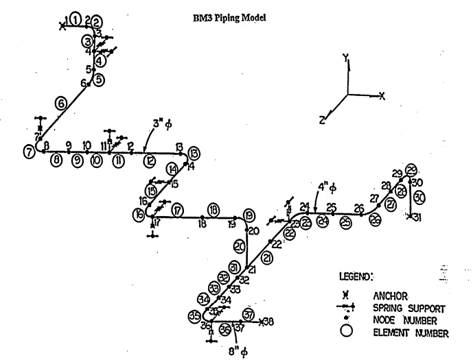
The geometry is wireframe. The following figure, taken from document [1], shows this geometry:

In order to compare correctly with American studies [1] and [2], the units chosen are imperial units.

The structure is composed of three parts with different sections. The following table shows the characteristics of the sections:

	Radius (inch)	Thickness (inch)
section 1	1.75	0.216
section 2	2.25	0.237
section 3	4.31	0.322

1.3. Meshing

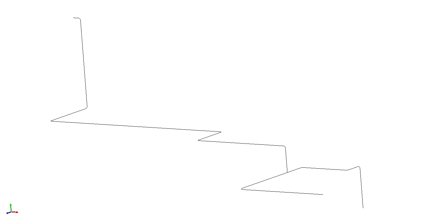
The structure’s mesh is linear and composed of 37 SEG2 elements for 38 nodes.

The following figure shows the mesh under SALOME - MECA -2012.1:

The following table shows the coordinates of the mesh nodes:

	Coordinates (inch)
Knots	\(X\)	\(Y\)	\(Z\)
1	0	0	0
2	15	0	0
3	19.5	-4.5	0
4	19.5	-180	0
5	19.5	-199,5	0
6	19.5	-204	4.5
7	19.5	-204	139.5
8	24	-204	144
9	96	-204	144
10	254	-204	144
11	333	-204	144
12	411	-204	144
13	483	-204	144
14	487.5	-204	148.5
15	487.5	-204	192
16	487.5	-204	235.5
17	492	-204	240
18	575	-204	240
19	723	-204	240
20	727.5	-208.5	240
21	727.5	-264	240
22	727.5	-264	205
23	727.5	-264	190
24	733.5	-264	184
25	753.5	-264	184
26	845.5	-264	184
27	851.5	-264	178
28	851.5	-264	160
29	851.5	-264	142
30	851.5	-270	136
31	851.5	-360	136
32	727.5	-264	255
33	727.5	-264	270
34	727.5	-264	306
35	727.5	-264	414
36	739.5	-264	426
37	847.5	-264	426
38	955.5	-264	426

The supports of this structure are modelled by stiffness. To be able to recover the nodal reactions to the supports, an additional « duplicate » node is created for each support. It is offset by \(\mathrm{1,E-3}\mathit{inch}\) (Code_Aster tolerance) along the \(X\) axis with respect to the support point. All its degrees of freedom are blocked and a SEG2 element is created between the support node and the « duplicate ». It is on this element that the values of the stiffness of the supports will be applied. Thus, the nodal reactions will be recorded at the « duplicate » nodes.

1.4. Materials

The material properties of the structure are as follows:

\(E\mathrm{=}\mathrm{2,9E+7}\mathit{pound}\mathrm{/}{\mathit{inch}}^{2}\)

\(\nu \mathrm{=}\mathrm{0,3}\)

The densities of the structure are as follows:

	Radius (inch)	Thickness (inch)	Thickness (inch)	Linear mass (pound/inch)	Thickness (inch)	Thickness (inch)
section 1	1.7500	0.216	0.216	2.2273	2.3240E-003	1.0434E-003
section 2	2.2500	0.237	0.237	3.1724	3.5145E-003	1.1078E-003
section 3	4.3125	0.322	0.322	8.3950	1.0836E-002	1.2908E-003

Note: In document [2] from 2010, the density in section 3 is \(1.253E\mathrm{-}3\mathit{pound}\mathrm{/}{\mathit{inch}}^{3}\). In order to maintain consistency in all models, the value of the 1999 document [1] is used.

1.5. Boundary conditions and loads

The boundary conditions correspond to the supports of the structure. They are modelled by stiffness at the corresponding nodes of the mesh. The stiffness is as follows:

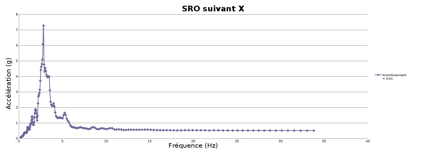
The loading of the spectral analysis corresponds to an Oscillator Response Spectrum applied in the \(X\) direction. The spectrum is shown in the following graph:

1.6. Modeling

Element POUTRE (2 models):

• modeling POU_D_T for straight sections and for curved sections

• DIS_TR modeling for supports