1. Reference problem#
1.1. Geometry#
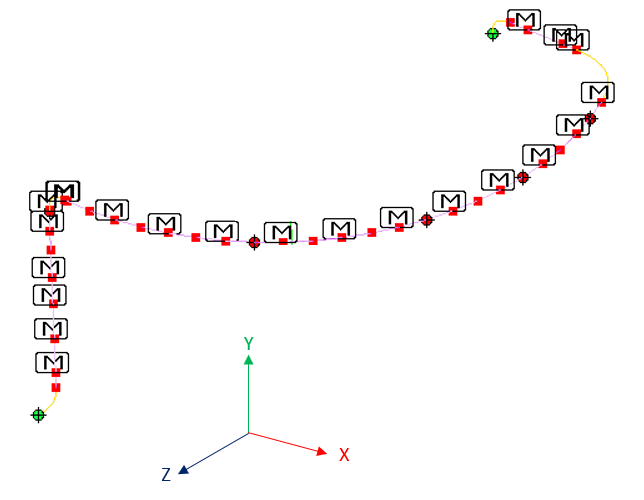
The pipe is modelled by a hollow circular section 762mm in diameter and 22mm thick (S1) or 813mm in diameter and 23mm thick (S2). The modeling is done with SEG2 (element POU_D_T) only.
Symbol |
Description |

|
Point mass |


|
0D spring in translation and/or rotation |
Figure 1: Benchmark 6 diagram
The following table shows the coordinates of each of the points in the pipe:
Knot |
X (m) |
Y (m) |
Z (m) |
PT_1 |
3.20 |
12.29 |
17.93 |
PT_2 |
3.20 |
12.29 |
17.90 |
PT_3 |
3.20 |
13.44 |
16.75 |
PT_4 |
3.20 |
14.43 |
16.75 |
PT_5 |
3.20 |
16.56 |
16.75 |
PT_6 |
3.20 |
18.69 |
16.75 |
PT_7 |
3.20 |
20.39 |
16.75 |
PT_8 |
3.20 |
22.08 |
16.75 |
PT_9 |
3.20 |
23.30 |
16.75 |
PT_10 |
3.20 |
24.52 |
16.75 |
PT_11 |
3.20 |
24.59 |
16.75 |
PT_12 |
4.31 |
25.74 |
16.50 |
PT_13 |
4.42 |
25.74 |
16.48 |
PT_14 |
5.84 |
25.74 |
16.03 |
PT_15 |
7.21 |
25.74 |
15.46 |
PT_16 |
8.53 |
25.74 |
14.77 |
PT_17 |
9.79 |
25.74 |
13.97 |
PT_18 |
10.97 |
25.74 |
13.07 |
PT_19 |
12.07 |
25.74 |
12.06 |
PT_20 |
13.08 |
25.74 |
10.96 |
PT_21 |
13.98 |
25.74 |
9.78 |
PT_22 |
14.78 |
25.74 |
8.52 |
PT_23 |
15.47 |
25.74 |
7.20 |
PT_24 |
16.04 |
25.74 |
5.83 |
PT_25 |
16.49 |
25.74 |
4.41 |
PT_26 |
16.81 |
25.74 |
2.95 |
PT_27 |
17.00 |
25.74 |
1.48 |
PT_28 |
17.07 |
25.74 |
-0.01 |
PT_29 |
17.00 |
25.74 |
-1.50 |
PT_30 |
16.81 |
25.74 |
-2.97 |
PT_31 |
16.49 |
25.74 |
-4.43 |
PT_32 |
16.04 |
25.74 |
-5.85 |
PT_33 |
15.47 |
25.74 |
-7.22 |
PT_34 |
14.78 |
25.74 |
-8.54 |
PT_35 |
13.99 |
25.74 |
-9.79 |
PT_36 |
9.53 |
25.74 |
-11.35 |
PT_37 |
8.78 |
25.74 |
-11.09 |
PT_38 |
6.66 |
25.74 |
-10.36 |
PT_39 |
5.63 |
25.74 |
-10.00 |
PT_40 |
4.55 |
24.59 |
-9.63 |
PT_41 |
4.55 |
24.59 |
-9.63 |
Table 1: Coordinates of pipe nodes
The following table shows the types of elements that make up the pipe:
Element |
Node 1 |
Node 2 |
Type |
Section |
EL_1 |
|
|
Tangent |
1 |
EL_2 |
|
|
Bend |
1 |
EL_3 |
|
|
Tangent |
1 |
EL_4 |
|
|
Tangent |
1 |
EL_5 |
|
|
Tangent |
1 |
EL_6 |
|
|
Tangent |
1 |
EL_7 |
|
|
Tangent |
1 |
EL_8 |
|
|
Tangent |
1 |
EL_9 |
|
|
Tangent |
1 |
EL_10 |
|
|
Tangent |
1 |
EL_11 |
|
|
Bend |
1 |
EL_12 |
|
|
Tangent |
1 |
EL_13 |
|
|
Tangent |
1 |
EL_14 |
|
|
Tangent |
1 |
EL_15 |
|
|
Tangent |
1 |
EL_16 |
|
|
Tangent |
1 |
EL_17 |
|
|
Tangent |
1 |
EL_18 |
|
|
Tangent |
1 |
EL_19 |
|
|
Tangent |
1 |
EL_20 |
|
|
Tangent |
1 |
EL_21 |
|
|
Tangent |
1 |
EL_22 |
|
|
Tangent |
1 |
EL_23 |
|
|
Tangent |
1 |
EL_24 |
|
|
Tangent |
1 |
EL_25 |
|
|
Tangent |
1 |
EL_26 |
|
|
Tangent |
1 |
EL_27 |
|
|
Tangent |
1 |
EL_28 |
|
|
Tangent |
1 |
EL_29 |
|
|
Tangent |
1 |
EL_30 |
|
|
Tangent |
1 |
EL_31 |
|
|
Tangent |
1 |
EL_32 |
|
|
Tangent |
1 |
EL_33 |
|
|
Tangent |
1 |
EL_34 |
|
|
Tangent |
1 |
EL_35 |
|
|
Bend |
1 |
EL_36 |
|
|
Tangent |
1 |
EL_37 |
|
|
Tangent |
1 |
EL_38 |
|
|
Tangent |
1 |
EL_39 |
|
|
Bend |
2 |
EL_40 |
|
|
Tangent |
2 |
Table 2: Type of pipe elements
1.2. Material properties#
The characteristics are as follows:
\(\mathit{YOUNG}=206000\mathit{MPa}\)
\(\mathit{NU}=0.30\)
\(\mathit{RHO}=0\mathit{kg}/m3\)
The mass of the pipe is not considered in this test case.
1.3. Boundary conditions and loads#
1.3.1. Boundary conditions#
In accordance with Figure, this study does not include fixed supports. On the other hand, some points are elastic supports whose characteristics are specified in the following tables:
Knot |
X (m) |
Y (m) |
Z (m) |
Type |
|
RESS_PT10_42_BASE |
0.00 |
0.00 |
0.00 |
-0.19 |
K_T_D_L |
RESS_PT10_43_BASE |
1.83 |
3.69 |
-0.03 |
K_T_D_L |
|
RESS_PT30_50_BASE |
2.78 |
3.69 |
3.69 |
0.92 |
K_T_D_L |
RESS_PT34_51_BASE |
2.75 |
3.71 |
3.00 |
K_T_D_L |
|
RESS_PT1_BASE |
3.20 |
12.29 |
12.29 |
17.93 |
K_ TR_D_L |
RESS_PT20_BASE |
13.08 |
25.74 |
25.74 |
10.96 |
K_ TR_D_L |
RESS_PT26_BASE |
16.81 |
25.74 |
2.95 |
K_ TR_D_L |
|
RESS_PT41_BASE |
4.55 |
24.59 |
-9.63 |
K_ TR_D_L |
Table 3: Coordinates and type of elastic supports
Node |
K local (N/m) |
K X (N/m) |
K Y (N/m) |
K Z (N/m) |
K RX (N/ rad )) ** |
K RY (N/ rad )) ** |
K RZ (N/ rad ) |
||
RESS_PT10_42_BASE |
1.75E+08 |
||||||||
RESS_PT10_43_BASE |
1.75E+08 |
||||||||
RESS_PT30_50_BASE |
3.50E+08 |
||||||||
RESS_PT34_51_BASE |
1.40E+08 |
||||||||
RESS_PT1_BASE |
1.75E+21 |
1.75E+21 |
1.75E+21 |
1.75E+21 |
1.75E+21 |
1.75E+21 |
1.75E+21 |
||
RESS_PT20_BASE |
4.37E+07 |
4.37E+07 |
3.50E+08 |
4.37E+07 |
|||||
RESS_PT26_BASE |
7.87E+07 |
3.50E+07 |
3.50E+08 |
7.87E+07 |
|||||
RESS_PT41_BASE |
1.75E+11 |
1.75E+11 |
1.75E+11 |
1.13E+16 |
1.13E+16 |
1.13E+16 |
1.13E+16 |
1.13E+16 |
Table 4: Stiffers of elastic supports
1.3.2. Loads#
The loads applied to the pipe are as follows:
Point masses in different nodes (identical in all 3 directions);
Earthquake in X, Y, and Z directions. The spectrum is weighted by 1 in all three directions;
Knot |
M ( kg ) |
PT_4 |
1 738.13 |
PT_5 |
954.97 |
PT_6 |
856.02 |
PT_7 |
1 031.15 |
PT_9 |
940.96 |
PT_11 |
691.75 |
PT_12 |
425.56 |
PT_13 |
690.17 |
PT_15 |
1 332.54 |
PT_17 |
1 332.54 |
PT_19 |
1 333.07 |
PT_21 |
1 332.89 |
PT_23 |
1 332.89 |
PT_25 |
1 332.89 |
PT_27 |
1 332.89 |
PT_29 |
1 332.89 |
PT_31 |
1 332.89 |
PT_33 |
1 331.14 |
PT_35 |
1 802.58 |
PT_36 |
1 316.60 |
PT_37 |
678.97 |
PT_38 |
1 843.74 |
Table 5: Values and locations of point masses
The spectra used for modal analysis are shown in the following figure:
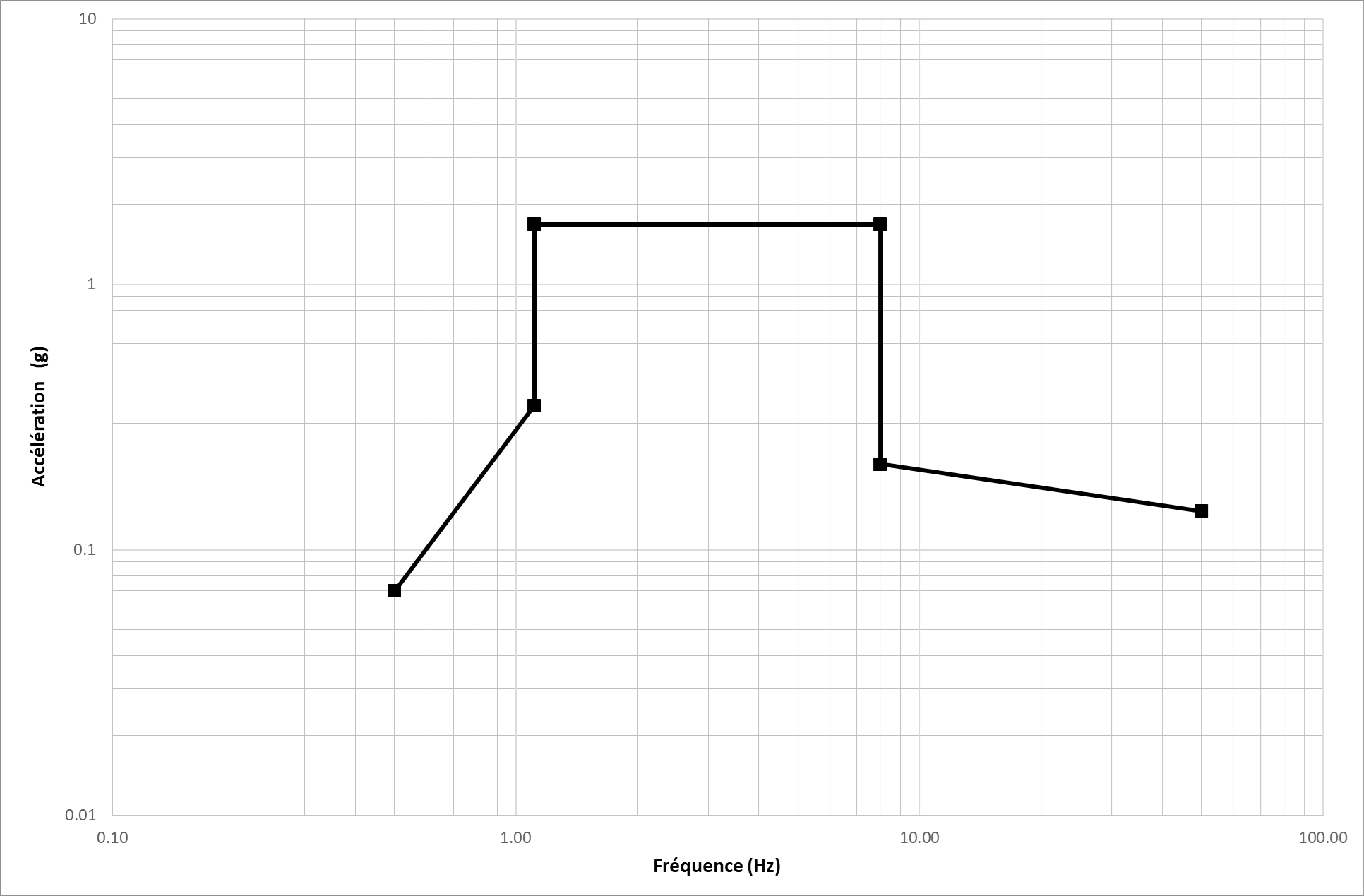
Figure 2: Computational spectrum — X and Z
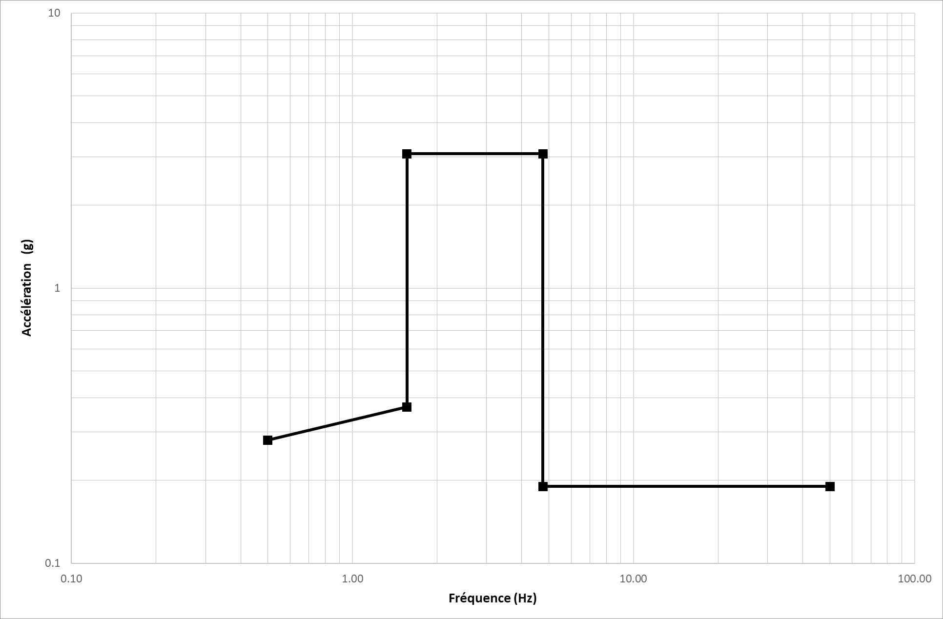
Figure 3: Computational spectrum - Y