3. Modeling A

3.1. Characteristics of modeling

Model A is modelled using elements DIS_T

3.2. Characteristics of the mesh

Number of knots: 2

Number of meshes: 3 DIS_T to model the mass (M_T_D_N), the stiffness (K_T_D_L) and the shock absorber (A_T_D_L)

3.3. Results

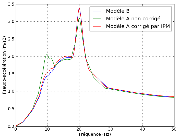
The vertical response spectrum obtained using the macro-command CALC_SPECTRE_IPM from the vertical acceleration of the node N 02 is compared to that obtained using the model B. We are in a case with relative coordinate resolution (single-press loading).

A check of the pseudo_acceleration values is performed for several acceleration values.

Node	Frequency	Reference	Reference Type	Tolerance
N02	5	0.425896	“AUTRE_ASTER”	3%
N02	10	1.44050	“AUTRE_ASTER”	3%
N02	15	1.93754	“AUTRE_ASTER”	0.1%
N02	20	3.39816	“AUTRE_ASTER”	0, 5%
N02	25	1.46011	“AUTRE_ASTER”	1%
N02	30	1.08058	“AUTRE_ASTER”	1.1%
N02	35	1.00117	“AUTRE_ASTER”	0, 9%
N02	40	0.929183	“AUTRE_ASTER”	0, 3%
N02	45	0.871687	“AUTRE_ASTER”	1%
N02	50	0.833936	“AUTRE_ASTER”	1, 9%

The treatment of the case is also validated in absolute reference, by comparison with the result in relation to a zero training signal.

Finally, we validate the initial correction (CORR_INIT =” OUI “) for which a non-zero initial acceleration is required. To do this, we will shift the training signal slightly in time: \(f(t)=\mathrm{sin}(2\mathrm{\pi }20.(t+0.00001))\). The answer obtained will therefore remain very close to the initial calculation without this delay.