2. Modeling A

2.1. Characteristics of modeling A

The first cut we’re testing corresponds to the case where one of the edges of TETRA10 sees the lsn cancel out exactly twice, at one of its ends and at its midpoint. An example of this configuration is shown in Figure.

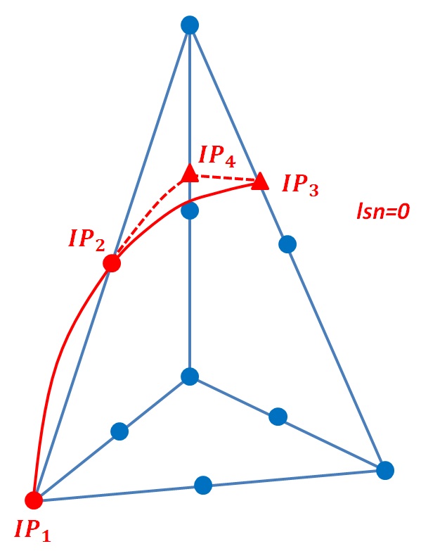
Figure 2.1-a : representation of the cut of modeling A

For cutting, we come back to the more classical case represented in Figure, whose sub-tetrahedron cutting is detailed in [R7.02.12].

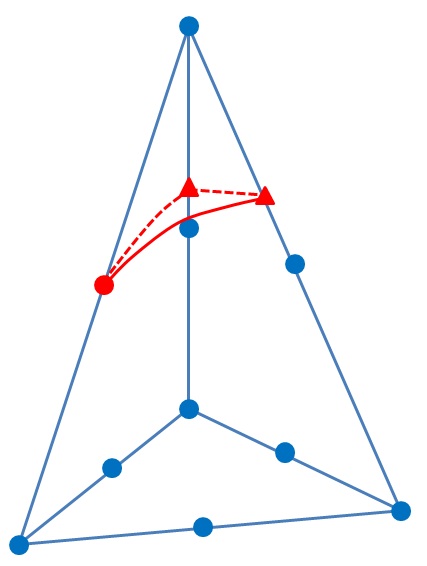
Figure 2.1-b : : corresponding healthy configuration

2.2. Characteristics of the mesh

To « find yourself » in this cutting configuration, the lsn is chosen spherical, with a center C (\(\frac{3}{4}\), \(\frac{3}{4}\), \(\frac{1}{4}\)) and with a radius \(R=\frac{\sqrt{(19)}}{4}\)

The edges of the tetrahedron are then intersected by the level set at the following 4 points:

Intersection point	Coordinates
IP1	(0,0,0)
IP2	(0,0,0.5)
IP3	(\(\frac{3-\sqrt{(5)}}{4}\) ,0, \(\frac{\sqrt{(5)}+1}{4}\))
IP4	(0, \(\frac{3-\sqrt{(5)}}{4}\), \(\frac{\sqrt{(5)}+1}{4}\))

2.3. Tested sizes and results

After executing command MODI_MODELE_XFEM, we check that the 4 intersection points IP1, IP2, IP3 and IP4 are in group NFISSU and that their position is correct.

Quantities tested	Reference type	Reference value	Tolerance
COORX IP1	“ANALYTIQUE”	0.0	10E-06
COORY IP1	“ANALYTIQUE”	0.0	10E-06
COORZ IP1	“ANALYTIQUE”	0.0	10E-06
COORX IP2	“ANALYTIQUE”	0.0	10E-06
COORY IP2	“ANALYTIQUE”	0.0	10E-06
COORZ IP2	“ANALYTIQUE”	0.5	10E-06
COORX IP3	“ANALYTIQUE”	0.19098300	10E-06
COORY IP3	“ANALYTIQUE”	0.0	10E-06
COORZ IP3	“ANALYTIQUE”	0.80901699	10E-06
COORX IP4	“ANALYTIQUE”	0.0	10E-06
COORY IP4	“ANALYTIQUE”	0.19098300	10E-06
COORZ IP4	“ANALYTIQUE”	0.80901699	10E-06

The cut mesh (Figure) was also post-processed using SALOME. The cut obtained is in accordance with expectations, with 4 subtetrahedra that are consistent with the discontinuity.

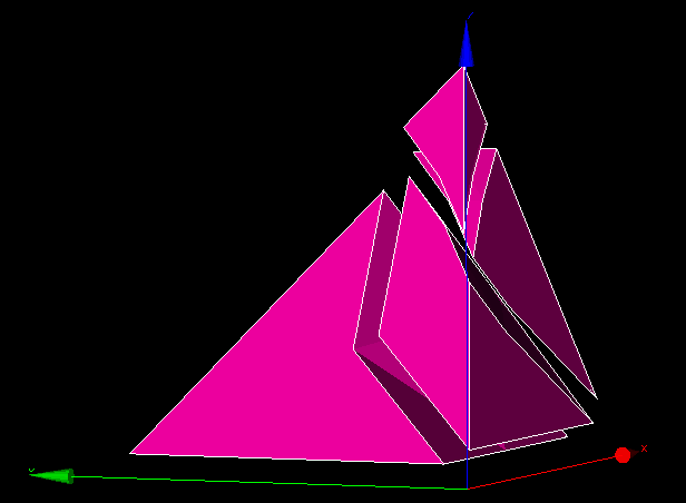
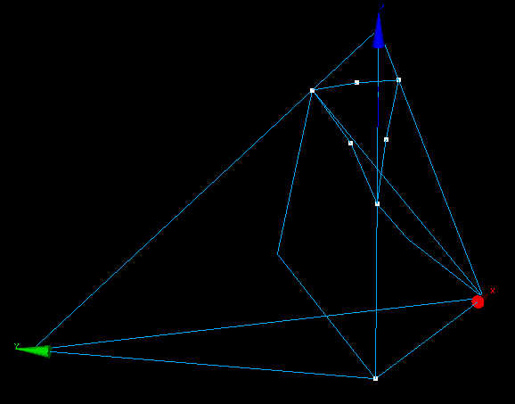
Figure 2.3-a : A modeling cutting configuration