2. Pairing process#
2.1. Fundamental dynamic equation of the rotating system#
The dynamic equation of the rotating system is written as follows (without taking into account prestress):
\(K\ddot{U}+(C+G)\dot{U}+(K+\mathit{KG})U=F\)
where:
\(M,C,K\): respectively the classical matrices of mass, damping and stiffness of the discretized system
\(G\mathit{et}\mathit{KG}\): respectively the Coriolis coupling and centrifugal stiffness matrices.
\(\ddot{U},\dot{U},U\): vectors in acceleration, speed and displacement
\(F\): external load vector
2.2. Part 1: Aster commands#
Aster commands are used to build the modal base. The mass, damping, gyroscopic and stiffness matrices are then projected onto this base.
The procedure for these orders is shown in the following flowchart:
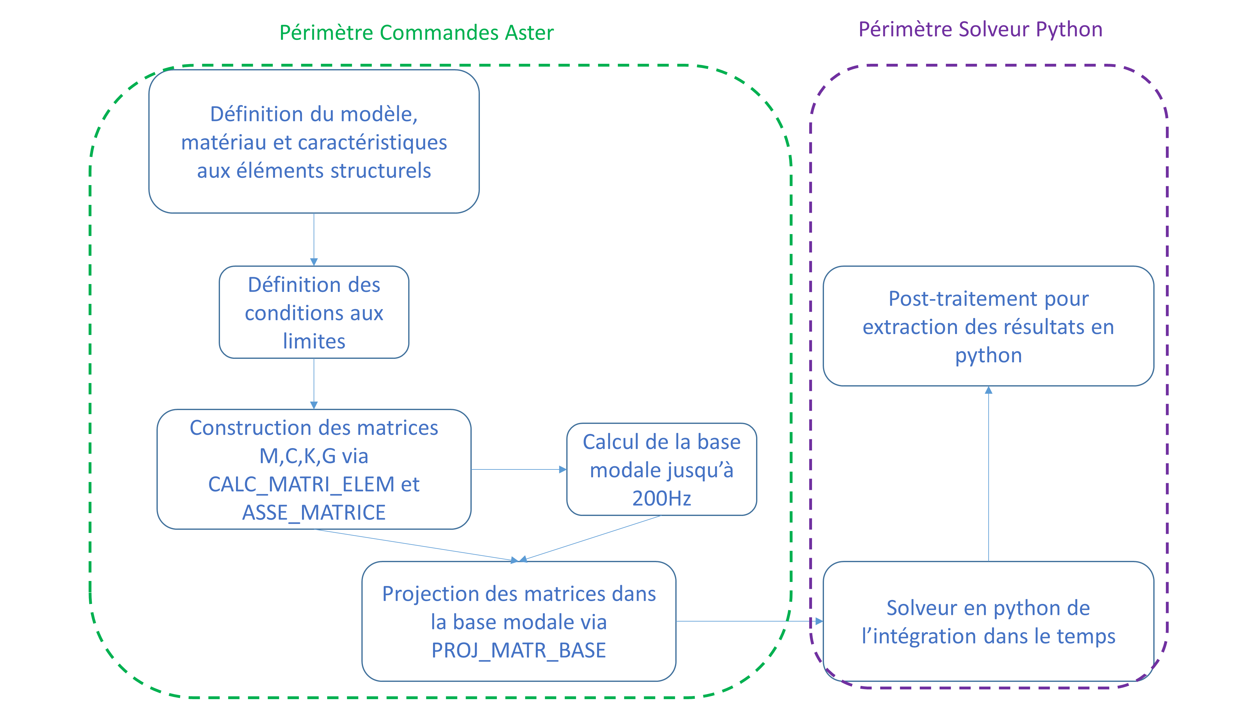
Figure 2.2-1
Matrixes are extracted and stored as objects in Python using the EXTR_MATR_GENE () command.
2.3. Part 2: Python Time Integration Solver#
The Python time integration solver uses the β-Newmark schema with γ=0.5 and β=0.25.
The solver architecture in Python is shown in the figure below:
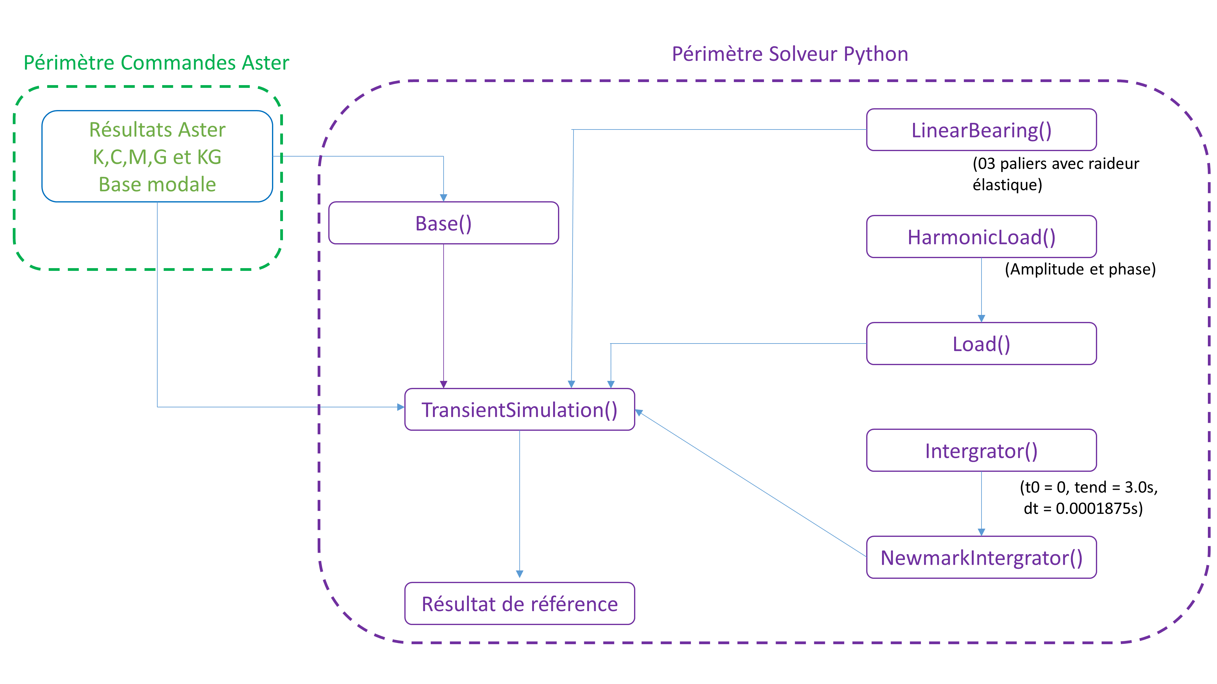
Figure 2.3-1
The classes are defined as follows:
Base (): convert Aster modal bases into Python language objects. This class makes it possible to convert result vectors from the generalized base to the physical base and vice versa;
Load (): generic class representing a loading;
linearBearing (): Allows linear bearings to be treated as an external loading. ;
HarmonicLoad (): Integrator harmonic load: Generic class representing a temporal integration schema.
newmarkIntegrator (): Integrator using the Newmark schema.
TransientSimulation (): Allows you to control the integration by building the loading vector and the archiving of the results.
The result obtained is the maximum value of the displacement in the N2Z1 node as a function of time.