2. B modeling#
2.1. Geometry#
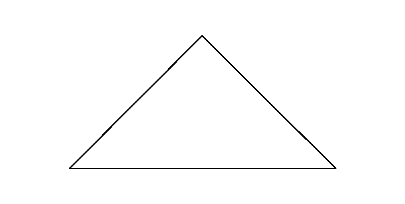
The geometry, shown in the following figure, is composed of a triangle with a base \(\mathrm{1m}\) and a height \(\mathrm{1m}\).
2.2. Characteristics of the mesh#
The mesh is 2D, quadratic and shown by the following figure:
It is composed of 6 knots for a TRIA6 stitch.
2.3. Adaptations made and resulting meshes#
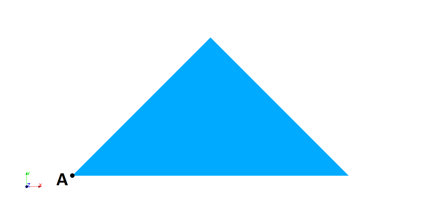
A field for movement at the nodes is created and the component \(\mathit{DX}\) is initialized to zero for all nodes, except node \(A\) (identified in the previous figure) for which \(\mathit{DX}\mathrm{=}1\).
Two uniform refinements are made with the displacement field updated. The first update is done with option CH_AUTO and the second with option CH_ISOP2. The expected updated field should therefore not be the same at the end of the two adaptations.
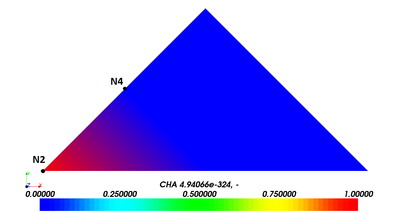
The following figure shows the initial field:
Note:
Validation, based on the updated field, will be performed on nodes 2 and 4. The value of \(\mathit{DX}\) in \(\mathit{N2}\) must be equal to 1 while in \(\mathit{N4}\) it is zero.
The following figure shows the field resulting from the adaptation with option CH_AUTO:
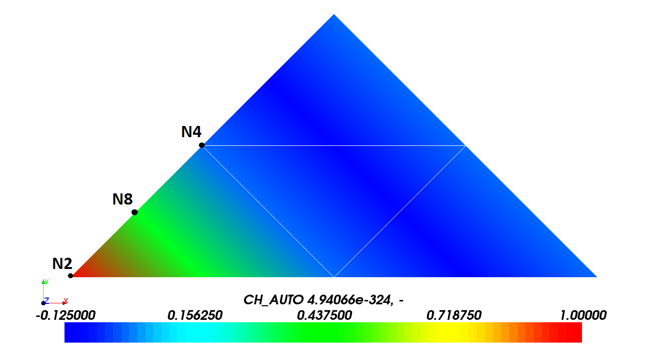
It appears, as expected, that the interpolated field does not respect the extreme values of the initial field (confer U7.03.01, §4.15.5).
Note:
Validation, based on the updated field, will be performed on nodes 2, 4 and 8. The values at nodes 2 and 4 should be the same as in the initial field. For node 8, with option CH_AUTO, the shape functions \(\mathit{P2}\), \({N}_{Ni}(i\mathrm{\in }\mathrm{[}\mathrm{1,6}\mathrm{]})\) (confer R3.01.01 §3.1) from the initial mesh are used for interpolation. So we expect to find: \({\mathit{DX}}_{\mathit{N8}}\mathrm{=}\mathrm{\sum }_{1}^{6}{\mathit{DX}}_{Ni}\mathrm{.}{N}_{Ni}({\xi }_{\mathit{N8}},{\eta }_{\mathit{N8}})\) for \({\xi }_{\mathit{N8}}\mathrm{=}1\mathrm{/}4\), \({\eta }_{\mathit{N8}}\mathrm{=}0\), \({\mathit{DX}}_{\mathit{N2}}\mathrm{=}1.\) and \({\mathit{DX}}_{Ni}\mathrm{=}0.(i\mathrm{\ne }2)\) for,, and i.e.: \({\mathit{DX}}_{\mathit{N8}}\mathrm{=}1.(\mathrm{-}(1.\mathrm{-}0.25)\mathrm{.}(1.\mathrm{-}2.(1.\mathrm{-}0.25)))\mathrm{=}0.375\).
The following figure shows the field resulting from the adaptation with option CH_ISOP2:
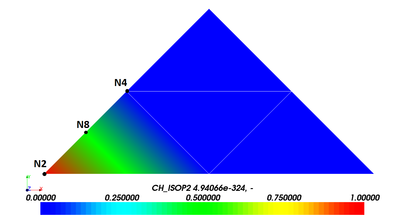
It appears, as expected, that with option CH_ISOP2, the interpolated field respects the extreme values of the initial field (confer U7.03.01, §4.15.5).
Note:
Nodes 2, 4, and 8 are identified because they are used for validation. The values at nodes 2 and 4 should be the same as in the initial field. For node 8, with option CH_ISOP2, functions of shapes \(\mathit{P1}\), \({N}_{Ni}(i\mathrm{\in }\mathrm{[}\mathrm{1,3}\mathrm{]})\) (confer R3.01.01 §3.1) expressed on the submeshes of the initial mesh element are used for interpolation. So we expect to find: \({\mathit{DX}}_{\mathit{N8}}\mathrm{=}\mathrm{\sum }_{1}^{3}{\mathit{DX}}_{Ni}\mathrm{.}{N}_{Ni}({\xi }_{\mathit{N8}},{\eta }_{\mathit{N8}})\) for \({\xi }_{\mathit{N8}}\mathrm{=}1\mathrm{/}2\), \({\eta }_{\mathit{N8}}\mathrm{=}0\), \({\mathit{DX}}_{\mathit{N2}}\mathrm{=}1.\) and \({\mathit{DX}}_{Ni}\mathrm{=}0.(i\mathrm{\ne }2)\) for,, and i.e.: \({\mathit{DX}}_{\mathit{N8}}\mathrm{=}1.(1.\mathrm{-}0.5)\mathrm{=}0.5\).
2.4. Tested sizes#
The following quantities are tested:
Initial Field |
Analytical Values |
Tolerance |
\(\mathit{N2}\) |
1.E-6 |
|
\(\mathit{N4}\) |
1.E-6 |
Field CH_AUTO |
Analytical Values |
Tolerance |
\(\mathit{N2}\) |
1.E-6 |
|
\(\mathit{N4}\) |
1.E-6 |
|
\(\mathit{N8}\) |
0.375 |
1.E-6 |
Field CH_ISOP2 |
Analytical Values |
Tolerance |
\(\mathit{N2}\) |
1.E-6 |
|
\(\mathit{N4}\) |
1.E-6 |
|
\(\mathit{N8}\) |
0.5 |
1.E-6 |