6. Order Details#
6.1. Case OPTION = “LONGUEUR”#
The cohesive crack is represented in FIG. 1, it is assumed to be rectilinear, and is divided into three distinct zones: healthy, cohesive (or damaged) and free surface (or cracked). The Gauss points (PG) of these zones are respectively represented in red, green and blue.
From these areas a cohesive point (white point) and a crack point (black point) are defined. The macro gives the distance between the origin point POINT_ORIG (red dot) and each of the two spikes in the direction and direction of the direction vector VECT_TANG (red vector) as well as the distance between the two spikes.
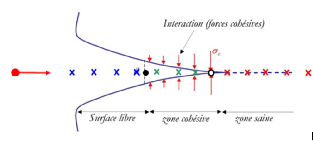
Figure1: Diagram of the cohesive crack and its Gauss points.
To define the position of the tips (see Figure 2) we rely on the geometric coordinates of the PGs and on the field of the internal variable VARI_ELGA component V3 of the laws CZM which takes as value 0 if the PG is healthy, 1 if the PG is damaged, 1 if the PG is damaged and 2 if the PG is cracked. For each of these three states we define Dmin and Dmax corresponding to the minimum and maximum distances with respect to the point of origin. The crack tip is positioned between the broken PGs and the damaged PGs, the cohesive tip is positioned between the damaged PGs and the healthy PGs.
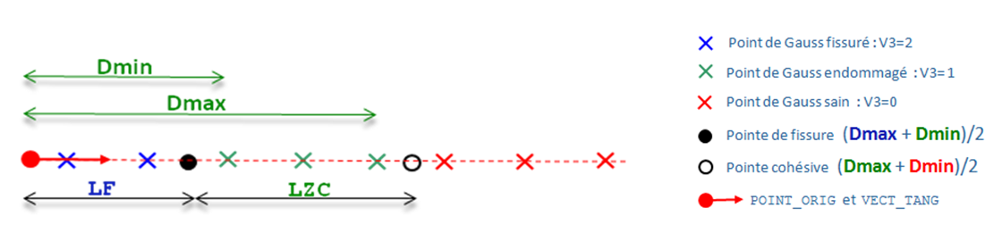
Figure2: Diagram of the PG field of a rectilinear 2D cohesive crack with the position of the tips (for example we plot Dmin and Dmax for damaged PGs).
6.2. Case OPTION = “TRIAXIALITE”#
For this option, the operation of the macro-command is as follows.
Detection of the presence of cohesive elements (see the models supported in the « scope of use » paragraph) in the model that was used to produce the evol_noli entered under the keyword RESULTAT. If no cohesive elements are detected, a fatal error message is issued.
Retrieving the constraint field corresponding to the last archived time step.
Making a loop on the meshes affected by cohesive elements. During this loop, for each cohesive cell, the cells of the massif that are directly adjacent to it (per face in 3D, and per edge in 2D) are identified using the sd_neighborhood data structure. We ensure that this cohesive cell has only one or two neighboring cells of this type (the zone of the mesh affected by the cohesive elements must therefore: either completely cross the structure, or be located on a part of the border as is for example the case when modeling a symmetry condition). Once these neighboring cells have been identified, the triaxiality rate of the stresses at all Gauss points of these neighboring elements is calculated. The arithmetic mean of the triaxiality at the Gauss points is then obtained: by elements and then on the number of neighbors if the current cohesive cell has 2 neighbors in the massif. Finally, in the map produced by the macro-command, the value of this averaged triaxiality is stored for the current cohesive mesh.
The map produced by the macro-command can then be used as a control variable in the operator AFFE_MATERIAU (AFFE_VARC/CHAM_GD) [U4.43.03] in order to vary the parameters of law cohesive with triaxiality.