11. Operand for nodal forces and reactions#

11.1. Operand FORCE#

| 'FORC_NODA'

Calculation of generalized nodal forces from the stresses at Gauss points. List of field components:

DX DY DZ	Nodal forces
Additional components for structural elements:
DRX DRY DRZ	Nodal forces (moments)

In the finite element sense, nodal forces correspond to the internal forces involved in the equilibrium equations. The calculation of generalized nodal forces \({F}_{K}\) is done as follows:

(11.1)#\[\sum _{K}{\mathrm{F}}_{K}\mathrm{.}{\mathrm{v}}_{K}={\int }_{\mathrm{\Omega }}\mathrm{\sigma }\mathrm{.}\mathrm{\epsilon }({\mathrm{v}}_{K})d\mathrm{\Omega }=\sum _{K}\underset{K}{\int }{\mathrm{\sigma }}^{K}\mathrm{.}\mathrm{\epsilon }({\mathrm{v}}_{K})\mathit{dK}=\sum _{K}\underset{K}{\int }{\mathrm{\sigma }}^{K}\mathrm{.}\mathrm{B}\mathrm{.}{\mathrm{v}}_{K}\mathit{dK}\]

With:

\({\mathrm{\sigma }}^{K}\) constraints at the Gauss points of element \(K\);
\(\mathrm{B}\) the generalized deformation finite element operator (matrix linking 1st order deformations to generalized displacements);
\({\mathrm{v}}_{K}\) generalized unit elementary displacement.

From where:

(11.2)#\[{\mathrm{F}}_{K}=\left\{\underset{K}{\int }{}^{t}\mathrm{B}\mathrm{.}{\mathrm{\sigma }}^{K}\mathit{dK}\right\}\]

The dimension of the nodal forces is dual to that of the \({v}_{K}\) to give a job (in Joules). For massive elements (3D, 2D and bars), FORC_NODA in general have the dimension of a force. This is a field on mesh nodes where the value in a node is obtained from the constraints calculated on the elements competing with this node, so their values therefore vary when the mesh changes. In the absence of distributed loading, equilibrium imposes their nullity in an internal node, while they correspond to the reaction on the supports where a kinematic relationship is imposed (case of an imposed displacement).

Two-dimensional case

For axisymmetric elements, the integration in \(\theta\) takes place on a sector of \(1\mathit{radian}\). If we want the integral of the surface force over the entire disk we must therefore multiply by \(2\pi\).

For elements in plane deformation, the calculation is done on a band of unit width. The calculated nodal forces are therefore in fact forces per unit length. If we want to calculate the nodal forces acting on a structure of width \(l\), we must multiply the result in D_PLAN by \(l\), except that the hypothesis of plane deformation is not valid in the vicinity of both faces. We will therefore have an approximate result.

Case of structural elements

For beam elements and discrete elements, the stresses at Gauss points are in fact the generalized nodal forces in the element coordinate system (obtained by the product of the element’s stiffness matrix by the displacement and taking into account thermal forces and distributed forces). The calculation of nodal forces is done by projecting the nodal forces contained in the symbolic name field “SIEF_ELGA” into the global coordinate system. The above summation of the elements then applies. The DX, DY, and DZ components give the strengths and DRX, DRY, and DRZ the moments.

In the case of shells, the components DX, DY and DZ give the FORC_NODA values (the dimensions of a force) in the global coordinate system of the mesh. These components are built with normal and sharp forces in the shell. The components DRX, DRY and DRZ give the FORC_NODA (moment dimensions) in the global coordinate system of the mesh, constructed with the bending moments in the shell. In the case of homogenized behaviors like ELAS_COQUE, it is best to look at EFGE_NOEU.

Two-dimensional case of thermo-hydro-mechanics (THM)

In (thermo-) hydro-mechanics, cf. §8, [R7.01.10], the generalized nodal forces associated with each component correspond to mechanical forces and flows. If we write \({Q}^{T}{\mathrm{\sigma }}_{0}\) the result of FORC_NODA, for hydraulic equations, then for a time step \(\Delta t\), we have:

(11.3)#\[\underset{\Omega }{\int }{Q}^{T}{\sigma }_{0}\cdot {p}^{\text{*}}d\Omega =-\Delta t\underset{\Omega }{\int }{M}^{-}\cdot \nabla {p}^{\text{*}}d\Omega\]

The flows are taken at time \({t}^{-}\) because of the \(\theta\) -schema used, cf. [R7.01.10].

If we note \(q\) the heat flow and \({M}_{w}\), \({M}_{\mathrm{vp}}\), \({M}_{\mathrm{as}}\) and \({M}_{\mathrm{ad}}\) the hydraulic flows of liquid water, steam, dry air (or any other component) and air dissolved in the liquid (these data correspond to the generalized constraints respectively \({M}_{1}^{1},{M}_{1}^{2},{M}_{2}^{1},{M}_{2}^{2}\), cf. §2.2, [R7.01.10]), then the expression of FORC_NODA is this:

The degree of freedom PRE1 in saturated, for example, is associated with the flow of water

(11.4)#\[-\Delta t\underset{\Omega }{\int }{({M}_{\mathrm{vp}}+{M}_{w})}^{-}\nabla {p}^{\text{*}}d\Omega\]

The flow of the gaseous component is associated with the unsaturated degree of freedom PRE2

(11.5)#\[-\Delta t\underset{\Omega }{\int }{({M}_{\mathrm{ad}}+{M}_{\mathrm{as}})}^{-}\cdot \nabla {p}^{\text{*}}d\Omega\]

The heat flow is associated with degree of freedom TEMP

(11.6)#\[-\Delta t\underset{\Omega }{\int }{q}^{-}\cdot \nabla {T}^{\text{*}}d\Omega\]

| 'REAC_NODA'

Calculation of the nodal forces of generalized reactions at the nodes, based on the stresses at the Gauss points and the loads. List of field components:

DX DY DZ	Nodal reactions
Additional components for structural elements:
DRX DRY DRZ	Nodal reactions (moments)

Generalized nodal reactions correspond in the sense of finite elements to the forces exerted on the supports (boundary conditions) participating in the equilibrium equations.

Static case

In statics, for result concepts such as evol_elas, mult_elas, mult_elas, fourier_elas or evol_noli, the calculation of generalized nodal reactions \({R}_{K}\) is done by:

(11.7)#\[\sum _{K}{\mathrm{R}}_{K}\mathrm{.}{\mathrm{v}}_{K}=\sum _{K}{\mathrm{F}}_{K}\mathrm{.}{\mathrm{v}}_{K}-\mathrm{L}({\mathrm{v}}_{K})\]

With:

\(\sum _{K}{\mathrm{F}}_{K}\mathrm{.}{\mathrm{v}}_{K}\) the expression of nodal forces (option FORC_NODA, see () and ());
\({v}_{K}\) generalized unit elementary displacement.

We have:

(11.8)#\[L({v}_{K})=\underset{\Omega }{\int }f\cdot {v}_{K}d\Omega +\underset{\Gamma }{\int }{F}_{s}\cdot {v}_{K}d\Gamma +\sum _{i}{F}_{i}\cdot {{v}_{K}}_{i}\]

With:

\(f\) are the volume forces;
\({F}_{s}\) generalized surface forces;
\({F}_{i}\) the generalized point forces at node \(i\).

The vector of the generalized nodal reactions on the element \(K\) is therefore obtained from the generalized nodal forces:

(11.9)#\[{\mathrm{R}}_{K}={\mathrm{F}}_{K}-\underset{K}{\int }\mathrm{f}\mathit{dK}-\underset{\partial K}{\int }\mathrm{F}\partial K-\sum _{i}{{\mathrm{F}}_{i}}_{K}\]

in other words, we subtract from the nodal forces the generalized external forces applied to the element \(K\).

note: Note that temperature loading does not appear in the external forces: it is involved in the expression of constraints via the law of behavior.

Case of non-linear transient dynamics

For evol_noli-type result concepts derived from non-linear transient dynamic calculations, in order to obtain nodal reactions, it is also necessary to remove inertia (acceleration) and damping forces related to speed:

(11.10)#\[\sum _{K}{\mathrm{R}}_{K}\mathrm{.}{\mathrm{v}}_{K}=\sum _{K}{\mathrm{F}}_{K}\mathrm{.}{\mathrm{v}}_{K}+(\mathrm{M}\ddot{\mathrm{u}})\cdot {\mathrm{v}}_{K}-\mathrm{L}({\mathrm{v}}_{K})\]

Where:

\(\sum _{K}{\mathrm{F}}_{K}\mathrm{.}{\mathrm{v}}_{K}\) the expression of nodal forces (option FORC_NODA, see () and ());
\({v}_{K}\) generalized unit elementary displacement.
\(M\) is the mass matrix;
\(\ddot{u}\) the generalized acceleration field;
\(L\) the vector of generalized external forces applied (equation ()).

notes

The contributions of damping directly related to speed on nodal reactions are overlooked;

The calculation of inertia forces requires the presence of the acceleration field ACCEdans the result data structure. In the case of an evol_noli-type structure, it is not possible for the code to verify its presence, so care should be taken.

Case of modal dynamics

For the result concepts of the mode_meca type (resulting from modal calculations) the formula is:

(11.11)#\[\sum _{K}{R}_{K}\mathrm{.}{v}_{K}=\underset{\Omega }{\int }\sigma (\varepsilon (u))\mathrm{.}\varepsilon ({v}_{K})d\Omega -{\omega }^{2}(M\cdot u)\cdot {v}_{K}\]

Where:

\(\sigma (\varepsilon (u))\) are the generalized modal constraints;
\(M\) is the mass matrix;
\(\omega\) the natural pulsation;
\(u\) the mode’s generalized travel field;
\({v}_{K}\) generalized unit elementary displacement.

Case of linear transient dynamics

For the result concepts of the dyna_trans type resulting from dynamic linear transient calculations (DYNA_VIBRA/TYPE_CALCUL =” TRAN “) or of the dyna_harmo type resulting from harmonic calculations (DYNA_VIBRA/TYPE_CALCUL =” HARM”) the expression of generalized nodal reactions is obtained by:

(11.12)#\[\sum _{K}{\mathrm{R}}_{K}\mathrm{.}{\mathrm{v}}_{K}=\sum _{K}{\mathrm{F}}_{K}\mathrm{.}{\mathrm{v}}_{K}+(\mathrm{M}\ddot{\mathrm{u}})\cdot {\mathrm{v}}_{K}-\mathrm{L}({\mathrm{v}}_{K})\]

Where:

\(\sum _{K}{\mathrm{F}}_{K}\mathrm{.}{\mathrm{v}}_{K}\) the expression of nodal forces (option FORC_NODA, see () and ());
\({v}_{K}\) generalized unit elementary displacement.
\(M\) is the mass matrix;
\(\ddot{u}\) the generalized acceleration field;
\(L\) the vector of generalized external forces applied (equation ()).

Use of GROUP_MA in FORC_NODA and REAC_NODA

If the keyword GROUP_MA is entered, \({F}_{K}\) (option FORC_NODA) is calculated only on the requested elements and then assembled. The result is different from a global calculation over the entire domain and then reduced to the required elements. The implemented method makes it possible to measure the reaction of one piece of model on another.

Attention! The calculation of “ REAC_NODA “ on a subset of the model (via the keyword GROUP_MA ) should be done with caution. Example 4 below illustrates this type of calculation.

For dyna_harmo results, the “REAC_NODA” is calculated only on the entire model. The calculation on a subset of the model can be done manually by calculating “FORC_NODA” on the group of elements in question and then subtracting the external force from the results obtained.

notes

The nodal reactions are zero at any point inside the model and are not zero a priory at a point on the edge subject to a kinematic boundary condition (or to contact forces);

Neglecting the contribution of damping dynamics may create a slight deviation from the exact result;

Only the resultant of nodal forces or reactions on a group of nodes makes physical sense (this group must correspond to at least one element of the model, for example an edge subject to a boundary condition). It can be calculated with POST_RELEVE_T [U4.81.21]. Occasionally, the FORC_NODA or REAC_NODA field should not be interpreted because the value in a node is directly linked to the fineness of the mesh. In addition, the sign of these forces on the nodes of the same element can be counterintuitive even though it is perfectly in agreement with finite element theory (for example on QUAD8situées cells at the interface of a zone in pure compression, the signs of the nodal forces at the vertices and in the midpoints are opposite);

The calculation of REAC_NODA takes into account the loads distributed over the beams. As soon as you vary this load on a non-linear calculation (change of EXCIT from one time step to another), the calculation of REAC_NODA is forbidden. It is necessary to divide its post-processing into « packages » of order numbers, for which the load is constant (i.e. it uses the same concept AFFE_CHAR_MECA in EXCIT).

Some loads are not taken into account when calculating this option, these are: INTE_ELEC, FORCE_SOL and RELA_CINE_BP.

11.2. Example 1: structure loaded with nodal force (2 elements QUAD4)#

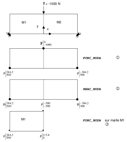
In this example, the reactions at nodes \((2)\) are indeed equal to the nodal forces \((1)\) minus the load. They represent the reactions to the supports of the structure.

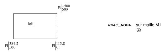
If we restrict the calculation to mesh \(\mathit{M1}\), the forces \((3)\) at the nodes belonging to the border between \(\mathit{M1}\) and \(\mathit{M2}\) are different. They represent the reaction of the model composed of \(\mathit{M1}\) to the model composed of \(\mathit{M2}\). Note that the nodal loading is divided by two because the two cells contribute to it. Nodal reactions \((4)\) are still equal to nodal forces minus loading.

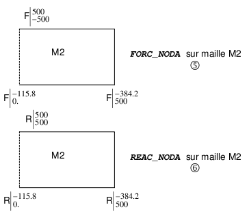
On the calculation restricted to cell \(\mathit{M2}\), the nodal forces \((5)\) following \(\mathit{OX}\) are of the opposite sign to the calculation restricted to cell \(\mathit{M1}\), illustrating the principle of action and reaction.

11.3. Example 2: structure with temperature loading#

Data:

\(E={1.10}^{9}\text{Pa}\)

\(\nu =0.3\)

\(\alpha ={1.10}^{-6}\)

Results:

\({F}_{y}=-{3.410}^{4}N\)

\({F}_{\mathrm{1x}}=7.8{10}^{3}N\)

\({F}_{\mathrm{2x}}=-1.2{10}^{3}N\)

In this example, the nodal forces and the nodal reactions coincide because the only loading is a loading temperature.

If we restrict the calculation to cell \(\mathit{M2}\), the forces following \(\mathit{OY}\) remain the same but are different according to \(\mathit{OX}\).

11.4. Example 3: structure under distributed load (beam)#

We consider a beam-type structure that is embedded and subjected to a loading of gravity on its upper half.

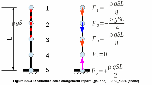
Figure 2.9.4-1: structure under distributed load (left), FORC_NODA (right)

On this type of structure, if we restrict the calculation of forces and nodal reactions to a subpart of the elements, FORC_NODA and REAC_NODA will not give the same result on the interface between the isolated part and the rest of the structure as shown in the figure (on force \({F}_{3}\)).

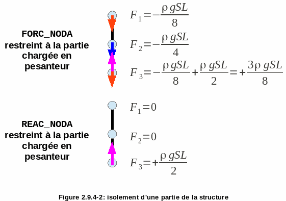
Figure 2.9.4-2: isolation of part of the structure

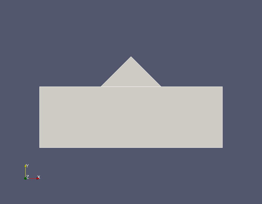
11.5. Example 4: Calculating the support reactions at the foot of a dam#

In this example, we schematize (very roughly!) a 2D dam. The dam is represented by a triangle DEF placed on a foundation represented by a rectangle ABCG (see diagram below).

We would like to calculate the support reactions of the dam on its foundation.

The loads are:

Gravity (which applies to the dam and its foundation)
Pressure loading due to the water reservoir (upstream side) applied on the CD and DE edges.
The foundation is embedded on AB.

In the following illustrations, the standard for field REAC_NODA has been represented when using the GROUP_MA keyword in various ways:

Illustration 1: we don’t use GROUP_MA (TOUT =” OUI “)
Figure 2: GROUP_MA =” BARRAGE “
Figure 3: GROUP_MA =( “BARRAGE”, “FROM”)
Figure 4: GROUP_MA =( “BARRAGE”, “DE”, “CD”)

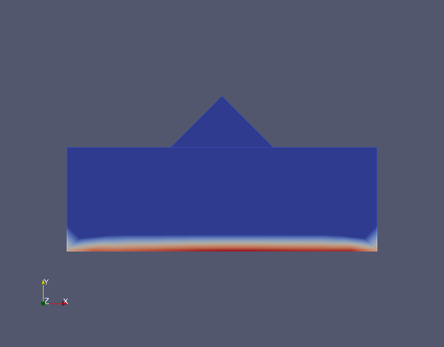
D E A GSchéma from B C F dam	Figure 1: REAC_NODA/TOUT =” OUI “



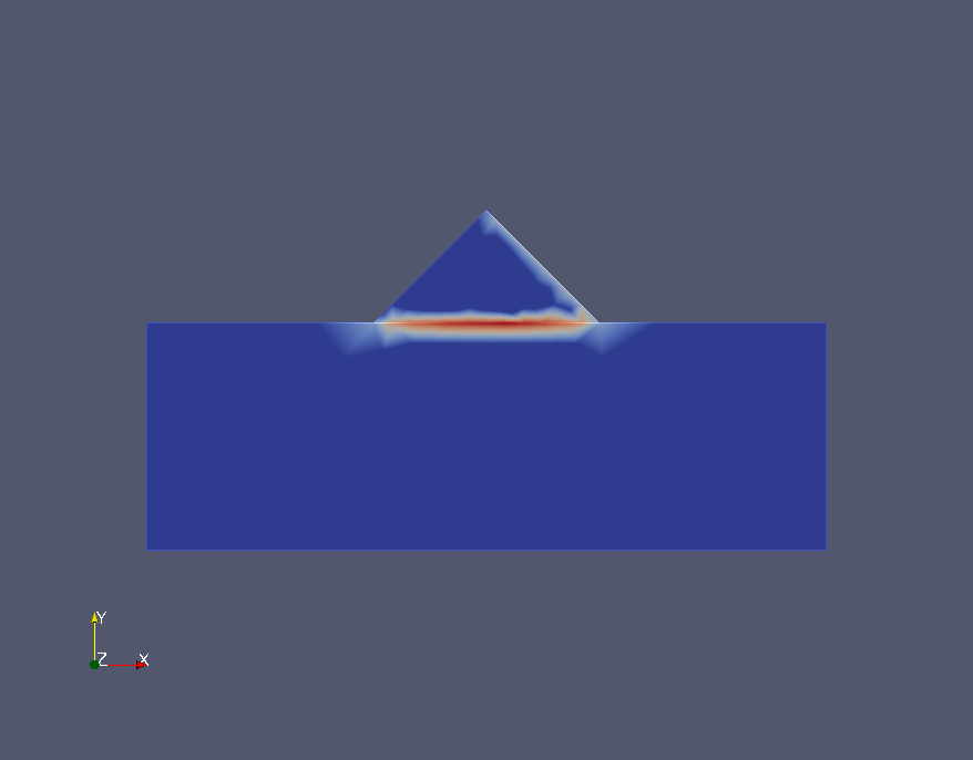
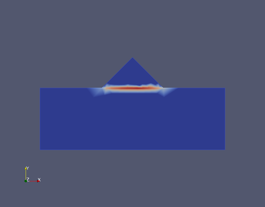
Picture 2: REAC_NODA/GROUP_MA =” BARRAGE “	Figure 3: REAC_NODA/GROUP_MA =( “BARRAGE”, “FROM”)



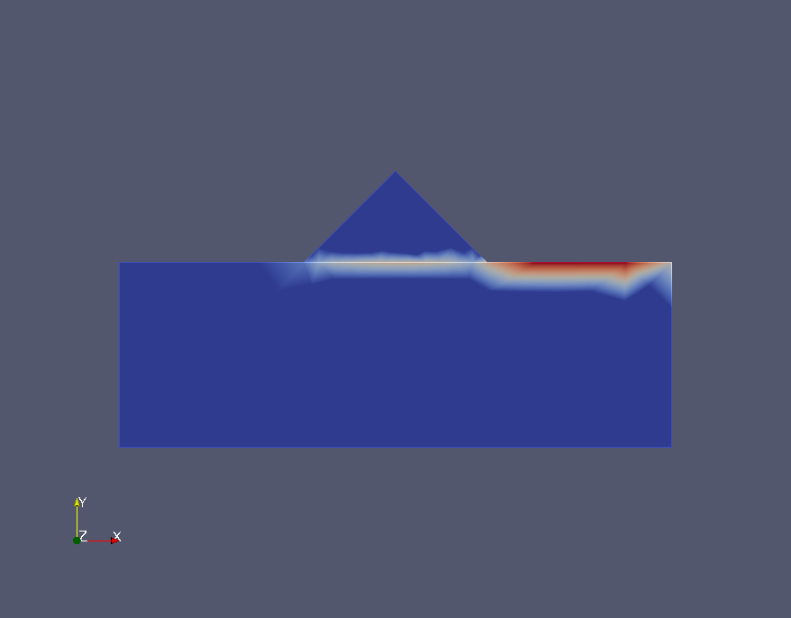
Figure 4: REAC_NODA/GROUP_MA =( “BARRAGE”, “DE”, “CD”)

Comments:

Illustration 1 shows that when the key word GROUP_MA is not used, the support reactions are non-zero only on the edge of the model where movements are imposed (here AB).
Illustration 2 shows that if we calculate REAC_NODA on the sole group BARRAGE (formed only of « volume » elements) non-zero reactions appear on DF (what we are looking for) but also on DE, which should alert us. The reason for this behavior is that the pressure load on DE has not been calculated, because the edge elements that calculate this load are not part of group BARRAGE.
Illustration 3 shows that if we calculate REAC_NODA on groups BARRAGE and DE, the reactions are the ones we are looking for: they are not zero only on DF. Note: the image seems to show that non-zero reactions exist on a portion of CD and FG, but this is an illusion due to visualization: the nodal forces at D and F « drool » on adjacent elements.
Figure 4 shows that you should not add too many edge groups (here CD). We can see that non-zero support reactions appear on CD. In this case, the reaction on point D is wrong.

Conclusion

If you want to calculate the support reactions of the dam on its foundation, you must ask for the calculation of REAC_NODA by specifying exactly all the cells of the dam and all the meshes of its edge subjected to a distributed loading.

It is strongly recommended to visualize the calculated reactions to verify that they are non-zero only at the interface between the dam and its foundation.