3. Operands

3.1. Principles

This operator solves the generalized problem (GEP) to the following eigenvalues [R5.01.01]:

Find \((\lambda ,\mathrm{x})\) such as \(\mathrm{A}\mathrm{x}\mathrm{=}\lambda \mathrm{B}\mathrm{x}\), \(\mathrm{x}\mathrm{\ne }0\), where \(\mathrm{A}\) and \(\mathrm{B}\) are real matrices, symmetric or not. To model hysteretic damping in the study of the free vibrations of a structure, the \(\mathrm{A}\) matrix can be complex symmetric [U2.06.03] [R5.05.04].

In mechanics, this type of problem corresponds in particular to:

• The study of the free vibrations of an undamped and non-rotating structure. For this structure, we look for the smallest eigenvalues or those that are in a given range to know if an excitatory force can create a resonance. In this case, the matrix \(\mathrm{A}\) is the material stiffness matrix, noted \(\mathrm{K}\), which is real symmetric (possibly increased by the geometric rigidity matrix marked \({\mathrm{K}}_{g}\), if the structure is prestressed), and \(\mathrm{B}\) is the mass or inertia matrix denoted by \(\mathrm{M}\) (real symmetric). The eigenvalues obtained are the squares of the pulsations associated with the frequencies sought. The system to be solved can be written

\(\underset{\mathrm{A}}{\underset{\underbrace{}}{(\mathrm{K}+{\mathrm{K}}_{g})}}\mathrm{x}\mathrm{=}\lambda \underset{\mathrm{B}}{\underset{\underbrace{}}{\mathrm{M}}}\mathrm{x}\)

where \(\lambda \mathrm{=}{(2\pi f)}^{2}\) is the square of the \(\omega\) pulse, \(f\) is the natural frequency, and \(\mathrm{x}\) is the associated natural displacement vector. The eigenmodes manipulated \((\lambda ,x)\) have real values. This type of problem is activated by the keyword TYPE_RESU =” DYNAMIQUE “and generates a data structure such as mode_meca, mode_acou or mode_gene (depending on the type of input data).

• The linear buckling mode research. In the framework of linearized theory, assuming a priori that stability phenomena are suitably described by the system of equations obtained by assuming the linear dependence of the displacement on the load level, the search for the x buckling mode associated with this critical load level \(\mu \mathrm{=}\text{-}\lambda\). This comes down to a generalized problem with the eigenvalues of the form:

\((\mathrm{K}+\mu {\mathrm{K}}_{g})x\mathrm{=}0\mathrm{\iff }\underset{\mathrm{A}}{\underset{\underbrace{}}{\mathrm{K}}}\mathrm{x}\mathrm{=}\lambda \underset{\mathrm{B}}{\underset{\underbrace{}}{{\mathrm{K}}_{g}}}\mathrm{x}\)

with \(\mathrm{K}\) material stiffness matrix and \({\mathrm{K}}_{g}\) geometric rigidity matrix. The eigenmodes manipulated \((\lambda ,x)\) have real values. This type of problem is activated by the keyword TYPE_RESU =” MODE_FLAMB “and generates a mode_flamb data structure.

Attention:

• In Code_Aster, we produce the eigenvalues of the generalized problem, * i.e. the variables \(\lambda\). To get the true critical loads, the variables \(\mu\) , you have to multiply them by —1.

Attention:

• In GEP, to deal with problems with complex modes (non-symmetric matrices and/or matrices with complex values), you must use the modal solver with METHODE =” SORENSEN “or” QZ “.

This operator also allows the study of the dynamic stability of a structure in the presence of damping and/or gyroscopic effects. This leads to the resolution of a higher-order modal problem, called quadratic (QEP) [R5.01.02]. We then look for complex eigenvectors and values \((\lambda ,\mathrm{x})\).

• The problem is finding \((\lambda ,\mathrm{x})\in (\mathrm{ℂ},{\mathrm{ℂ}}^{N})\) such as:

\(({\lambda }^{2}\mathrm{B}+\lambda \mathrm{C}+\mathrm{A})\mathrm{x}\mathrm{=}0\)

where typically, in linear mechanics, \(\mathrm{A}\) will be the stiffness matrix, \(\mathrm{B}\) the mass matrix and \(\mathrm{C}\) the damping matrix. The matrices \(\mathrm{A}\), \(\mathrm{B}\), and \(\mathrm{C}\) are symmetric and real matrices. The complex eigenvalue \(\lambda\) is related to the natural frequency \(f\) and to the damping reduced by \(\xi\) by \(\lambda \mathrm{=}\xi (2\pi f)\mathrm{\pm }i(2\pi f)\sqrt{1\mathrm{-}{\xi }^{2}}\). This type of problem is activated by the keyword TYPE_RESU =” DYNAMIQUE “and generates a mode_meca_c data structure.

Attention:

• In QEP, to deal with problems with non-symmetric matrices and/or complex values, you must use the modal solver with METHODE =” SORENSEN “or” QZ “.

• Buckling ( TYPE_RESU =” MODE_FLAMB “) is not legal in QEP.

• **Sturm test*

  [R5.01.04] `_ < https://code-aster.org/V2/doc/default/fr/man_r/r5/r5.01.04.pdf>*only operates in GEP with real symmetric matrices. Outside this framework (QEP, GEP with real non-symmetric matrices or with matrix* :math:`A symmetric complex), the “BANDE” option is forbidden and post-verification based on Sturm test is not activated (parameter VERI_MODE/STURMinopérant) .

To solve these generalized or quadratic modal problems, Code_Aster offers various approaches. Beyond their numerical and functional specificities, which are included in the documents [R5.01.01] [R5.01.02], they can be summarized in the form of the table below (the values by default are shown in bold).

Operator/ Scope of application	Algorithm	Keyword	Benefits	Disadvantages
Reverse power method OPTION = “ SEPARE “, “ AJUSTE “, “or”PROCHE”**		OPTION =			*Only real symmetric (GEP and QEP) . *
1**er*phase (heuristic)
Calculating some modes	Bissection (not applicable in QEP) .	“ SEPARE “
Calculating some modes	Bissection+ Secant (GEP) or Muller Traub (QEP) .	“ AJUSTE “	Better accuracy	Cost calculation
Improvement of some estimates	User initialization	“ PROCHE “	Resumption of eigenvalues estimated by another process. Cost: calculation of this phase is almost zero	No capture of the multiplicity of modes
2**th*phase (inverse power method)						Only real symmetric (GEP and QEP)
Basic method	Inverse powers	“ DIRECT “	Very good eigenvector construction	Not very robust
Acceleration option	Rayleigh quotient
(not applicable in QEP) »	“ RAYLEIGH “	Improve convergence	Cost calculation
Simultaneous iteration method OPTION = “ PLUS_ * “, “ CENTRE “, “ BANDE “ or “ TOUT “		SOLVEUR_MODAL = _F (METHODE =
Calculating part of the spectrum	Bathe & Wilson	“ JACOBI “		Not very robust Real symmetric only (GEP)
	Lanczos (Newman-Pipano in GEP and Jennings in QEP)	“ TRI_DIAG “	Specific detection of rigid modes.	Only real symmetric (GEP and QEP)
	IRAM (Sorensen)	“ SORENSEN “	Increased robustness. Better computing and memory complexities. Fashion quality control.	Method by default. Accessible symmetric and non-symmetric and with \(\mathrm{A}\) symmetric complex or real*.*
Calculating the entire spectrum and then filtering part of it.	QZ	“ QZ “	Reference method in terms of robustness.	Very expensive in CPU and in memory. To be reserved for small cases (<103 degrees of freedom). Accessible in symmetric and in not symmetric and with \(\mathrm{A}\) symmetric complex or real .

Table 3.1-1 - Summary of Code_Aster modal methods

To capture a significant portion of the spectrum, it is best to use the values” PLUS_PETITE “**”** “, “ PLUS_GRANDE “, **” CENTRE “, or**” BANDE “of the keyword OPTION, , which use a « simultaneous iterations » » values that use a « simultaneous iterations » method **: subspace methods (Lanczos, IRAM, Jacobi) or the global QZ method (very robust but expensive method; to be booked to small problems).

On the other hand, when it comes to determining a few simple well-discriminated eigenvalues or refining some estimates, the values “ SEPARE “, “ AJUSTE “or “ PROCHE “ of the keyword OPTION (which use a method such as « inverse powers ») are often well indicated.

It is also highly recommended to take advantage of the strengths of the two classes of methods by refining the eigenvectors obtained beforehand by a method of simultaneous iterations, via the inverse power method . This will reduce the norm of the final residue. This is what the post-processing keyword “AMELIORATION” allows you to do, cf. §3.13.

Thus, even if the options for simultaneous iteration methods (” PLUS_PETITE/GRANDE “,”/”, , “”, ,) are often preferable, one can calculate up to ten modes with the options of power-type methods: “SEPARE”, “AJUSTE” or “PROCHE”. CENTRE BANDE To calculate dozens or even hundreds of modes, it is necessary to use the “BANDE” option when possible. This improves the robustness, quality, and performance of the compute.

In the standard case of a real symmetric GEP, ideally you should organize your calculation into several sub-bands, each comprising between 20 and 60 modes. With, if possible, a homogeneous division into the number of modes (an « imbalance » of less than 3 [1]). ).

To do this, we can proceed in several steps:

• Calibrate the areas of interest by an initial call to INFO_MODE [U4.52.01] on a [2] frequency list

(resp. critical loads) given,

• Look the number of eigenmodes displayed in the message file (or in the generated sd_table),

• Relaunch one or more CALC_MODES calculations with OPTION =” BANDE “by trying to balance the bands.

Note :

• If we finally calculate only one band, to save time, we can even pool part of the calculation cost of the initial INFO_MODE by notifying to CALC_MODES the name of the sd_table generated (cf. keywords TABLE_). This chaining can thus make the additional cost of *INFO_MODE*negligible and guide the modal calculation effectively. *

On the other hand, as soon as we treat an atypical QEP or GEP (complex and/or non-symmetric matrix), the spectrum becomes complex. The INFO_MODE + CALC_MODES chaining is then no longer possible. Some keywords or values become irrelevant (OPTION =” BANDE “, VERI_MODE/STURM…).

Note :

• It is strongly recommended that you first read the reference documentation [R5.01.01] [R5.01.02] and [R5.01.04]. It gives the user the properties and limitations, theoretical and practical, of the modal methods addressed while relating these considerations to the precise parameterization of the options.

3.2. Keyword TYPE_RESU

◊ TYPE_RESU = /' DYNAMIQUE '[DEFAUT]

/” MODE_FLAMB “ /” GENERAL “

This keyword makes it possible to define the nature of the modal problem to be treated: search for vibration frequencies (classical case of dynamics with or without damping and gyroscopic effects) or search for critical loads (case of linear buckling theory, only in GEP). Depending on this class of membership, the results are displayed and stored differently in the data structure:

• In dynamics (TYPE_RESU =” DYNAMIQUE “, the frequencies are ordered in increasing order of the modulus of their shift deviation (cf. [R5.01.01/02], §3.8/2.5). It is the value of the access variable NUME_ORDRE of the data structure. The other access variable, NUME_MODE, is equal to the true modal position in the eigenvalue spectrum (determined by the Sturm test cf. [R5.01.04]). This Sturm test is only legal in GEP with real modes (real symmetric matrices), in other cases (GEP with complex modes and QEP), we set NUME_MODE = NUME_ORDRE.

• In buckling (TYPE_RESU =” MODE_FLAMB “), the eigenvalues are stored in increasing algebraic order. The variables NUME_ORDRE and NUME_MODE take the same value equal to this order.

• General case (TYPE_RESU =” GENERAL “): same as for the buckling case.

Note :

• The TYPE_RESU =” GENERAL “solves a problem a ux*eigenvalues in the case of a* **general matrix system. For the moment its perimeter is limited to standard GEPs (symmetric real matrices). Its only difference with* MODE_FLAMB is therefore only in the naming of the matrices: MATR_A/MATR_B rather than MATR_RIGI/MATR_RIGI_GEOM ..

3.3. Operand CHAM_MATER

◊ CHAM_MATER = chmat


Material field name.

3.4. Operand CARA_ELEM

◊ CARA_ELEM = character


Name of the characteristics of the elements of beams, shells, etc.

3.5. Operands MATR_RIGI/MATR_A/MATR_MASS/MATR_RIGI_GEOM//MATR_B/MATR_AMOR

The table below represents the operands to use according to the type of keyword TYPE_RESU.

TYPE_RESU
“DYNAMIQUE”	“MODE_FLAMB”	“GENERAL”
♦ MATR_RIGI = A	♦ MATR_RIGI = A	♦ MATR_A = A
♦ MATR_MASS = B	♦ MATR_RIGI_GEOM = B	♦ MATR_B = B
◊ MATR_AMOR = C	Not applicable	Outside the current perimeter

Table 3.5-1 - Name of the input matrices according to TYPE_RESU

♦ MATR_RIGI/MATR_A = A

Assembled matrix, real (symmetric or not) or symmetric complex, of the type [Matr_asse_*_R/C] of the GEP/QEP to be solved.

♦ MATR_MASS/MATR_RIGI_GEOM/MATR_B = B

Assembled matrix, real (symmetric or not), of type [Matr_asse_*_R] of the GEP/QEP to be solved.

◊ MATR_AMOR = C

Assembled matrix, real (symmetric or not), of type [Matr_asse_*_R] of the QEP to be solved.

Note :

If the matrix A*is symmetric complex or if one of the matrixs* A, B*or* C*is not symmetric real, only certain sets of parameters are allowed. In particular:*

- the options “BANDE” , “PROCHE” , “ “, “ SEPARE” , “AJUSTE “are not usable

- if A is complex: “PLUS_PETITE” is not usable, ni “CENTRE “if the target frequency is 0

- the resolution methods “ JACOBI “and” TRI_DIAG “(in SOLVEUR_MODAL/METHODE ) are not usable.

3.6. Operand OPTION

◊ OPTION=

“BANDE”	We are looking for all the eigenvalues in a given band. This band is defined by the argument of FREQ = \(({f}_{\mathit{min}},{f}_{\mathit{max}})\) or by that of CHAR_CRIT = \(({\lambda }_{\mathit{min}},{\lambda }_{\mathit{max}})\) . Option only available in GEP with symmetric real matrices. In the case TYPE_RESU =” DYNAMIQUE “, the keyword FREQpeut be a list of n>2 values: FREQ = \(({f}_{1}={f}_{\mathit{min}},,\mathrm{...},{f}_{i},\mathrm{...},{f}_{n}={f}_{\mathit{max}})\). In this case, the global search band is divided into almost independent sub-bands \([{f}_{i},{f}_{i+1}]\) (cf. §:ref:).
“CENTRE”	We are looking for the NMAX_FREQvaleurs proper ones closest to the frequency \(f\) (keyword argument FREQ = \(f\)) or the NMAX_CHAR_CRITcharges criticisms closest to the load \(\lambda\) (keyword argument CHAR_CRIT = \(\lambda\)).
“ PLUS_PETITE “ [DEFAUT]	We are looking for the NMAX_FREQplus small natural frequencies (case TYPE_RESU =” DYNAMIQUE “) or the NMAX_CHAR_CRITplus small critical loads (TYPE_RESU =” MODE_FLAMB “or” GENERAL “).
“PLUS_GRANDE”	We are looking for the NMAX_FREQplus major eigenvalues. Option usable only in the case TYPE_RESU =” DYNAMIQUE “, for a generalized problem, with symmetric real matrices. The roles of stiffness and mass matrices are interchanged in a way that is transparent to the user. Note: It may be useful to disable the STURM test in the VERI_MODE operand. Indeed, at the heart of the algorithm, before being converted into physical natural frequencies, the eigenvalues can be very small and very similar.
“TOUT”	We’re looking for all the modes associated with physical degrees of freedom. Option usable only with the ModalQZ solver (cf. §:ref:).
“PROCHE”	We look for the modes whose eigenvalues are closest to the given values. These values are indicated by: the lfreq argument of the FREQ keyword for a dynamic GEP (TYPE_RESU =” DYNAMIQUE “). the argument lcharc of the CHAR_CRIT keyword for a linear buckling GEP (TYPE_RESU =” MODE_FLAMB “). the arguments lfreqet lamordes the keywords FREQ and AMOR_REDUITpour a QEP of dynamic type (TYPE_RESU =” DYNAMIQUE “). There are as many fashion searches as there are terms in this list (or these lists). Note: If you want to calculate a multiple mode, you should not use this option because you will only find one mode for each given value in the list.
“SEPARE”	The eigenvalues are separated by a bisection method based on the Sturm criterion. The limits of the search interval are: the values of the list lfreq of the FREQ keyword for a generalized or quadratic dynamic problem (TYPE_RESU =” DYNAMIQUE “). the values in the list lcharcu the CHAR_CRITpour keyword is a generalized linear buckling problem (TYPE_RESU = “MODE_FLAMB”).
“AJUSTE”	Operation similar to the previous” SEPARE “option. After separating the natural frequencies via the “SEPARE” option (in GEP only), additional iterations are carried out either by the secant method (GEP) or by the Müller-Traub method (QEP) to obtain better precision on the eigenvalues.

Table 3.6-1 **- Possible keyword values OPTION

It is important to remember that choosing one of these options involves the use of a particular method:

• OPTION =” BANDE “,” CENTRE “,” “,” PLUS_PETITE “,” “,” “,” PLUS_GRANDE “or “TOUT” involves the use of a method of simultaneous iterations

  • • OPTION =” PROCHE “,” SEPARE “,” “,” AJUSTE “involves the use of the inverse power method.

This choice has consequences on the rest of the keywords available in the command, in particular on the SOLVEUR_MODAL configuration.

See [R5.01.01/02] §2.5/3.8.

3.7. Keyword factor SOLVEUR_MODAL

Keyword used to adjust the algorithms and parameters of the modal solver.

3.7.1. Keywords associated with the method of simultaneous iterations

These keywords can only be used if the value of the OPTION keyword is among “PLUS_PETITE”, “”, “PLUS_GRANDE”, “BANDE”, “CENTRE”, “TOUT”.

3.7.1.1. Keyword METHODE

Four resolution methods are then available to solve the problem with eigenvalues (cf. also):

◊ METHODE =/' SORENSEN '[DEFAUT]

We use the Sorensen method (external package ARPACK) to calculate the eigenmodes of GEP or QEP (cf. [R5.01.01/02] §7/4). Its perimeter includes real matrices, symmetric or not, or even a complex symmetric \(A\) matrix.

/”TRI_DIAG”

We use the Lanczos method (variant of Newmann-Pipano in GEP, of Parlett & Saad in QEP) to calculate the eigenmodes of GEP or QEP (cf. [R5.01.01/02] §6/4). Its perimeter is limited to real symmetric matrices.

/”JACOBI”

We use the Bathe & Wilson method (then the Jacobi method on the projected system) to calculate the eigenmodes of GEP (cf. [R5.01.01] §8). Its perimeter is limited to real symmetric matrices.

/”QZ”

We use the QZ method from the external library LAPACK to calculate the eigenmodes of GEP or QEP (cf. [R5.01.01/02] §9/5). Its perimeter includes real matrices, symmetric or not, or even a complex symmetric \(\mathrm{A}\) matrix. This very expensive reference method should be reserved for problems of small size (<103 degrees of freedom).

3.7.1.2. Parameters related to the resolution method

Each of these resolution methods has different settings:

• if METHODE =” SORENSEN “:

◊ PREC_SOREN =pso (0.) [DEFAUT]

Note:

• The method then considers that it must work with the smallest possible precision, the « zero machine ». To have an order of magnitude, in double precision on standard machines, this value is close to \(2.22{.10}^{-16}\) .

◊ NMAX_ITER_SOREN =NSO (20) [DEFAUT]

◊ PARA_ORTHO_SOREN =porso (0.717) [DEFAUT]

These are parameters for adjusting the required precision on the modes (by default, machine precision is chosen), the authorized number of restarts of the Sorensen method (cf. [R5.01.01] §7) and the orthogonalization coefficient of the IGSM of Kahan-Parlett (see [R5.01.01] appendix 2).

If the porso coefficient is negative, the reorthogonalization is performed on all the calculated modes instead of targeting only the modes belonging to the same clean space. The calculation can then be two or three times more expensive.

For more information on how to select clean spaces, you can consult the SEUIL_FREQ/CHAR_CRIT parameters.

Note:

• During the first few runs, it is strongly recommended not to change these advanced parameters of the algorithm, which are initialized empirically to standard values.

• if METHODE =” TRI_DIAG “:

◊ PREC_ORTHO =po (1.10-12) [DEFAUT]

◊ NMAX_ITER_ORTHO =nio (5) [DEFAUT]

◊ PREC_LANCZOS =pl (1.10-8) [DEFAUT]

◊ NMAX_ITER_QR =name (30) [DEFAUT]

◊ MODE_RIGIDE =/” OUI “

/” NON “[DEFAUT]

The first two parameters make it possible, respectively, to adjust the precision of orthogonalization and the number of reorthogonalizations in the Lanczos method to obtain independent vectors generating the subspace (cf. [R5.01.01] §6).

The third is an adjustment parameter for determining the nullity of a term on the superdiagonal of the tridiagonal matrix characterizing the reduced problem obtained by the Lanczos method. It is just a deflation criterion and not, contrary to what its name might suggest, a criterion for the quality of fashion.

The fourth sets the maximum number of iterations for solving the reduced system for the QR method ([R5.01.01] appendix 1).

The keyword MODE_RIGIDE makes it possible to detect and calculate in advance, by an algebraic method, rigid body modes. They are then used to calculate the other modes with the Lanczos algorithm. They are provided to the user only if they are part of the requested modes. If rigid body modes are calculated without using this option, the eigenvalues calculated by the Lanczos algorithm are not zero but very close to zero.

Note :

• During the first few steps, it is strongly recommended not to modify these parameters, which rather concern the arcana of the algorithm and which are initialized empirically to standard values.

• if METHODE =” JACOBI “:

◊ PREC_BATHE =pbat (1.10-10) [DEFAUT]

◊ NMAX_ITER_BATHE =nbat (40) [DEFAUT]

◊ PREC_JACOBI =Pjaco (1.10-2) [DEFAUT]

◊ NMAX_ITER_JACOBI =njaco (12) [DEFAUT]

The first two parameters allow, respectively, to adjust the convergence precision and the maximum number of iterations allowed of the Bathe & Wilson method (cf. [R5.01.01] §8).

The other two adjust the precision of the convergence and the maximum number of iterations of the JACOBI method (cf. [R5.01.01] appendix 3). This global modal solver is used to calculate the eigenmodes of the projected matrix according to the DeBathe & Wilson algorithm.

Note :

• During the first few steps, it is strongly recommended not to modify these parameters, which rather concern the arcana of the algorithm and which are initialized empirically to standard values.

• if METHODE =”QZ”:

◊ TYPE_QZ = /' QZ_SIMPLE '[DEFAUT]

/” QZ_EQUI “ /” QZ_QR “

This parameter allows you to choose one of the variants of the QZ algorithm proposed by LAPACK. The first choice (“QZ_SIMPLE”) designates the basic method, the second (“QZ_EQUI”) adds pre-processing to balance the terms of the matrix. This often improves the quality of the modes but, conversely, if the matrix has very small terms due to rounding errors, this phase then generates parasitic modes.

As for the third choice (“QZ_QR”), it is reserved for the positive definite symmetric case (real stiffness matrix, Dirichlet condition without Lagrange, no buckling or damping step). It is much faster than the previous options.

3.7.1.3. Keyword APPROCHE

◊ APPROCHE = /' REEL '[DEFAUT]

/” IMAG “ /” COMPLEXE “(only with Sorensen)

This keyword defines the type of approach (real, imaginary or complex) for choosing the scalar pseudo-product of QEP used with the Lanczos method or with that of Sorensen (cf. [R5.01.02]).

This operand only makes sense for the analysis of vibrations (TYPE_RESU =” DYNAMIQUE “) free of a damped or rotating structure (complex natural modes; the keyword MATR_AMOR must be entered). In buckling, (TYPE_RESU =” MODE_FLAMB “) this is of no interest.

Notes:

• In quadratic, with the Lanczos method only the “ IMAG “ approach is compatible with a zero frequency limit (” OPTION = PLUS_PETITE “or “ CENTRE “ with \(f=0\) ) .

• With Sorensen, none are compatible.

3.7.1.4. Keywords DIM_SOUS_ESPACE and COEF_SOUS_ESPACE

◊ DIM_SOUS_ESPACE =some

◊ COEF_DIM_ESPACE =MSE

EXCLUS (“DIM_SOUS_ESPACE”, “COEF_DIM_ESPACE”)

If the DIM_SOUS_ESPACE keyword is not entered or is initialized to a value strictly less than the number of requested frequencies nf, the operator automatically calculates an admissible dimension for the projection subspace using COEF_DIM_ESPACE (cf. § 5 of this document and [R5.01.01] §5.3).

Thanks to the data of this multiplying factor, MSE, we can project onto a space whose size is proportional to the number of frequencies contained in the study interval.

If we are looking for specific modes on a band divided into several sub-bands (OPTION =” BANDE “and FREQ is a list of at least 3 values), we can therefore optimize the size of the subspaces which remains proportional to the number of frequencies sought on each sub-band: the sub-spaces rich in eigenvalues thus do not penalize the poorest ones (in terms of CPU).

However, the size of this subspace can be set arbitrarily, via the value taken by the DIM_SOUS_ESPACE keyword (which must be greater than nf to be taken into account).

In both cases, if the size of the projection subspace ndim is strictly greater than the number of « active degrees of freedom », nactive (cf. [R5.01.01] §3.2), then it is forced to take this ceiling value.

Remarks :

• If we use the Sorensen method (IRAM) and ndim-nf < 2 , numerical-computer imperatives force to impose ndim=nf+2.

In quadratic, we work on a real problem of double size: 2*nf, 2*ndim*.*

• These parameters are useless for the “ QZ “ method .

3.7.2. Parameters associated with the inverse power method

These parameters are therefore only available if the value of the OPTION keyword is among “PROCHE”, “SEPARE”, “AJUSTE”.

3.7.2.1. Bisection operands (if OPTION =” SEPARE “or” AJUSTE “)

◊ NMAX_ITER_SEPARE=nis (30) [DEFAUT] ◊ PREC_SEPARE =ps (1.10-4) [DEFAUT]

Parameters for adjusting the number of iterations and separation accuracy for dichotomy research. These operands are ignored for the “PROCHE” option (Cf. [R5.01.01] §4.2).

3.7.2.2. Secant operands (if OPTION =” AJUSTE “)

◊ NMAX_ITER_AJUSTE = nia (15) [DEFAUT] ◊ PREC_AJUSTE = pa (1.10-4) [DEFAUT]

Parameters for adjusting the number of iterations and the separation precision for the secant method. These operands are only used for the “AJUSTE” option (Cf. [R5.01.01] §4.2).

Note :

During the first few steps, it is strongly recommended not to modify these parameters, which rather concern the arcana of the algorithm and which are initialized empirically to standard values.

3.7.2.3. Calculation parameters of the second phase of calculation of the inverse power method

◊ OPTION_INV =/” DIRECT “ [DEFAUT]

/”RAYLEIGH”

Definition of the inverse power method (cf. [R5.01.01/02] §4.3/3.3):

“ DIRECT “ [DEFAUT]	standard method in GEP or variant of Jennings in QEP.
“RAYLEIGH”	Acceleration via Rayleigh quotient (only in GEP)

Table 3.7.2.3-1 - Operation of OPTION_INV according to its value

◊ NMAX_ITER_INV=nim (30) [DEFAUT]

Maximum number of iterations of the inverse power method for the search for natural modes.

◊ PREC_INV=pm (1.10-5) [DEFAUT]

Stop test of the inverse power method.

3.8. Keyword factor CALC_FREQ (if TYPE_RESU =” DYNAMIQUE “)

◊ CALC_FREQ =_F (...

Keyword factor that specifies the parameters for calculating the natural modes and their number, depending on the OPTION chosen.

3.8.1. Operand FREQ (only if OPTION =” BANDE “or” “or” CENTRE “or” “or” PROCHE “or” SEPARE “or” AJUSTE “)

♦ FREQ =l_f

◊ TABLE_FREQ =table_f

List of frequencies: its use depends on the OPTION chosen.

OPTION =” BANDE “	We expect a list of \(n\ge 2\) \(({f}_{\mathit{min}}={f}_{1},\mathrm{...},{f}_{i},\mathrm{...},{f}_{\mathit{max}}={f}_{n})\) values that define the search band. If n > 2, the global search band \([{f}_{\mathit{min}},{f}_{\mathit{max}}]\) is divided into sub-bands \([{f}_{i},{f}_{i+1}]\).
OPTION =” CENTRE “	We expect only one frequency value.
OPTION =” PROCHE “	We expect a list of \(n\ge 1\) values \(({f}_{1},\mathrm{...},{f}_{i},\mathrm{...}{f}_{n})\) that define the frequencies around which we are looking for the closest natural frequency.
OPTION =” SEPARE “ or “AJUSTE”	We expect a list of \(n\ge 2\) \(({f}_{1},\mathrm{...},{f}_{i},\mathrm{...}{f}_{n})\) values that define the boundaries of the search intervals \([{f}_{i},{f}_{i+1}]\).

Table 3.8.1-1 - Use of the keyword FREQ depending on the OPTION chosen

• With the “BANDE” option: the values specified under this keyword must be positive and strictly increasing.

---

• If \(n=2\):

we start by operating a Sturm test in order to determine the number of modes contained in the band (cf. [R5.01.04]). If we have previously calibrated the area of interest with a INFO_MODE, we can save part of this calculation cost. To do this, we reuse the table generated by INFO_MODE, which we fill in with the keyword: TABLE_FREQ =table_f. The terminals \(({f}_{\mathit{min}},{f}_{\mathit{max}})\) defined above make it possible to select one or more rows from said table.

For example, if the table was generated by a:

INFO_MODE with a list FREQ = \(({f}_{\mathit{im0}},{f}_{\mathit{im1}},{f}_{\mathit{im2}},{f}_{\mathit{im3}},{f}_{\mathit{im4}},{f}_{\mathit{im5}})\),

we can share part of the calculated cost by setting in CALC_MODES with the option “BANDE”: FREQ = \(({f}_{\mathit{min}}={f}_{\mathit{im1}},{f}_{\mathit{max}}={f}_{\mathit{im4}})\). The preprocessing step of CALC_MODES will then not perform the Sturm test but, instead, detect in the table the sub-bands included in the interval. So here:

\([{f}_{\mathit{im1}},{f}_{\mathit{im2}}]\cup [:ref:`{f}_{\mathit{im2}},{f}_{\mathit{im3}} <{f}_{\mathit{im2}},{f}_{\mathit{im3}}>\)]cup [{f}_{mathit{im3}},{f}_{mathit{im4}}] `.

We will then just sum the numbers of modes corresponding to each sub-interval in order to derive/to establish the total number of modes to search for.

This chaining really makes it possible to reduce the additional cost of initial calibration by INFO_MODE and is therefore to be used whenever possible.

Notes about chaining of INFO_MODE commands **** with CALC_MODES **** and option “ BANDE “:

• The selection boxes \(({f}_{\mathit{min}},{f}_{\mathit{max}})\) must correspond exactly to those used to generate the INFO_MODEinitial (with VERI_MODE/PREC_SHIFT%) [3]

) .

• The rows in the table are selected based on the initial values of the frequencies. But if they have experienced offsets (because the boundaries were too close to eigenvalues), the table also traces these values after offsets (values FREQ_MIN/MAX/ [4]

). It is of course these last offset values that are transmitted to the algorithm of CALC_MODES. This strategy thus preserves, at the same time, the ergonomics of the option and the consistency of the software behaviors: a CALC_MODES * and option “ BANDE “provides the same result, whether it starts its preprocessing phase with or without a pre-calculated table.

• If one of the selection terminals had to be offset (in the previous INFO_MODE), the pre-processing phase emits a ALARMEpour to reproduce the same behavior as for a standard calculation.

• The table table_f must have no holes or covers, otherwise it is rejected. But this scenario cannot normally happen with a card from INFO_MODE. This rule makes it possible to preserve the robustness of the algorithmic scheme: we don’t want to miss any frequency.

• If \(n>2\):

the calibration of each sub-band by the operator INFO_MODE is done automatically within the operator CALC_MODES. In addition, searches on each of the sub-bands can be parallelized in order to reduce calculation times (cf. § 3.14).

Notes:

• Each frequency is treated only once: as the lower bound of the first sub-band for the first in the list, as the upper bound of the following sub-bands for the other frequencies. In particular, if this frequency is considered too close to an eigenvalue, it is offset ( cf. [U4.52.01] and [R5.01.04]).

• The possible offset of a frequency terminal only occurs once in INFO_MODEinitial. Therefore, there is no risk of the overlap of staggered intervals. There is therefore no risk of calculating the same mode twice by mistake.

• With the “PROCHE” option: the values specified under this keyword must be positive and strictly increasing. this is the list of frequencies whose mode we are looking for the nearest mode.

• With the “SEPARE” or “AJUSTE” option: the values are the limits of the search intervals. We will try to separate the frequencies in the intervals:

[f *1* ,f2], [f2, f3]… [f*n* -2, f*n* -1], [f*n* -1, f*n*]

The list has at least two items. Frequencies should be positive and in ascending order.

3.8.2. Operand AMOR_REDUIT (only if OPTION =” CENTRE “or” PROCHE “)

◊ AMOR_REDUIT =l_a

Reduced damping value that allows you to define the complex eigenvalue (the « shift ») around which the closest eigenvalues are sought (cf. [R5.01.01] §5.4). This option can only be used in the context of a modal problem with complex modes: QEP or GEP with non-symmetric real matrices or with a symmetric complex \(\mathrm{A}\).

OPTION =” CENTRE “	We expect only one reduced depreciation value
OPTION =” PROCHE “	We expect a list of reduced depreciation values, of the same size as the list given under the FREQ keyword.

Table 3.8.2-1 - functioning of the keyword AMOR_REDUIT depending on the OPTION chosen

The value specified under this keyword must be positive and between 0 and 1.

3.8.3. Operand NMAX_FREQ (only if OPTION =” PLUS_PETITE “or” “or” PLUS_GRANDE “or” “or” CENTRE “or” SEPARE “or” AJUSTE “)

◊ NMAX_FREQ =nf (10 if OPTION =' PLUS_PETITE ', 1 if OPTION =' PLUS_GRANDE', 0 if OPTION =' SEPARE 'or' AJUSTE ') [DEFAUT]

Maximum number of eigenvalues to be calculated.

• If OPTION =” PLUS_PETITE “or” PLUS_GRANDE “or” CENTRE “:

If nf is strictly greater than the number of active « degrees of freedom » nactive (cf. [R5.01.01] §3.2), then it is forced to take this ceiling value.

• If OPTION =” PROCHE “:

The value is ignored.

• If OPTION =” SEPARE “or” AJUSTE “:

If the user does not enter this keyword, all the eigenvalues contained in the intervals specified by the user are calculated. Otherwise, the first NMAX_FREQ eigenvalues, and therefore the lowest ones, are calculated.

3.9. Keyword factor CALC_CHAR_CRIT (if TYPE_RESU =” MODE_FLAMB “or” GENERAL “)

◊ CALC_CHAR_CRIT =_F (...

Keyword factor that specifies the parameters for calculating the natural modes and their number, depending on the OPTION chosen.

3.9.1. Operand CHAR_CRIT (only if OPTION =” BANDE “or” “or” CENTRE “or” “or” PROCHE “or” SEPARE “or” AJUSTE “)

♦ CHAR_CRIT =l_c

◊ TABLE_CHAR_CRIT =table_c

List of critical loads: its use depends on the option chosen.

OPTION =” BANDE “	We expect two \(({\lambda }_{\mathit{min}},{\lambda }_{\mathit{max}})\) values that define the search band
OPTION =” CENTRE “	We expect only one critical load value
OPTION =” PROCHE “	We’re waiting for a list of \(n\ge 1\) values that define the \(({\lambda }_{\mathrm{1,}}{\lambda }_{\mathrm{2,}}\mathrm{...},{\lambda }_{n\mathrm{-}1},{\lambda }_{n})\) charges around which we’re looking for the closest critical load.
OPTION =” SEPARE “ or “AJUSTE”	We expect a list of \(n\ge 2\) values that define the \(({\lambda }_{\mathrm{1,}}{\lambda }_{\mathrm{2,}}\mathrm{...},{\lambda }_{n\mathrm{-}1},{\lambda }_{n})\) bounds of the search intervals \([{\lambda }_{i},{\lambda }_{i+1}]\).

Table 3.9.1-1 - Use of the keyword CHAR_CRIT depending on the OPTION chosen

The values specified under this keyword are positive or negative. In QEP it is of no interest.

• With the “BANDE” option, we start by running a Sturm test in order to determine the number of modes contained in the band (see [R5.01.04]). If we have previously calibrated the area of interest with a INFO_MODE, we can save part of this calculation cost. To do this, we reuse the table_c table generated by INFO_MODE. The terminals \(({\lambda }_{\mathit{min}},{\lambda }_{\mathit{max}})\) defined above make it possible to select one or more rows from said table.

For example, if the table was generated by a

INFO_MODE + CHAR_CRIT = \(({\lambda }_{\mathit{im0}},{\lambda }_{\mathit{im1}},{\lambda }_{\mathit{im2}},{\lambda }_{\mathit{im3}},{\lambda }_{\mathit{im4}},{\lambda }_{\mathit{im5}})\),

we can share part of the calculated cost by setting in CALC_MODES +” BANDE “, CHAR_CRIT = \(({\lambda }_{\mathit{min}}={\lambda }_{\mathit{im1}},{\lambda }_{\mathit{max}}={\lambda }_{\mathit{im4}})\). The pre-processing step in CALC_MODES will then not perform the Sturm test but, instead, detect in the table_c table the sub-bands included in the interval. So, here:

\([{\lambda }_{\mathit{im1}},{\lambda }_{\mathit{im2}}]\cup [:ref:`{\lambda }_{\mathit{im2}},{\lambda }_{\mathit{im3}} <{\lambda }_{\mathit{im2}},{\lambda }_{\mathit{im3}}>\)]cup [{lambda }_{mathit{im3}},{lambda }_{mathit{im4}}] `.

We will then just sum the numbers of modes corresponding to each sub-interval in order to derive/to establish the total number of modes to search for.

This chaining really makes it possible to reduce the additional cost of initial calibration by INFO_MODE and is therefore to be used whenever possible.

Notes about chaining **** INFO_MODE **** with the option CALC_MODES +” BANDE “:

• The selection boxes \(({\lambda }_{\mathit{min}},{\lambda }_{\mathit{max}})\) must correspond exactly to those used to generate the table table_cdel” INFO_MODEinitial (with VERI_MODE/PREC_SHIFT%) %* [5]

) .

• The rows in the table table_c are selected in relation to the initial values of the frequencies. But if they have experienced offsets (because the boundaries were too close to eigenvalues), the table also traces these values after offsets (values CHAR_CRIT_MIN/MAX/ [6]

). It is of course these last offset values that are transmitted to the algorithm of CALC_MODES. This strategy thus preserves both the ergonomics of the option and the consistency of the software behaviors: a CALC_MODES with the option “BANDE” provides the same result, whether it starts its pre-processing phase with or without a precalculated table.

• If one of the selection terminals had to be offset (in the table table_c de l” INFO_MODEpréalable), the pre-processing phase emits a ALARMEpour to reproduce the same behavior as for a standard calculation.

• The table table_chas to have no holes or covers, otherwise it is rejected. But this scenario cannot normally happen with a table table_cissue of INFO_MODE. This rule makes it possible to preserve the robustness of the algorithmic scheme: we don’t want to miss any frequency.

• With the “PROCHE” option: the values specified under this keyword must be positive and strictly increasing. This is the list of critical loads whose closest buckling mode is being sought.

• With the “SEPARE” or “AJUSTE” option: the values are the limits of the search intervals. We will try to separate the critical loads in the intervals:

\(\mathrm{[}{\lambda }_{\mathrm{1,}}{\lambda }_{2}\mathrm{]},\mathrm{[}{\lambda }_{\mathrm{2,}}{\lambda }_{3}\mathrm{]}\mathrm{...}\mathrm{[}{\lambda }_{n\mathrm{-}2},{\lambda }_{n\mathrm{-}1}\mathrm{]},\mathrm{[}{\lambda }_{n\mathrm{-}1},{\lambda }_{n}\mathrm{]}\)

The list has at least two items. Critical loads should be positive and in ascending order.

3.9.2. Operand NMAX_CHAR_CRIT (only if OPTION =” PLUS_PETITE “or” “or” CENTRE “or” SEPARE “or” AJUSTE “)

◊ NMAX_CHAR_CRIT =nf (10) [DEFAUT]

Maximum number of critical loads to be calculated.

• If OPTION =” PLUS_PETITE “or” CENTRE “:

If nf is strictly greater than the number of « active degrees of freedom », nactive (cf. [R5.01.01] §3.2), then it is forced to take this ceiling value.

• If OPTION =” PROCHE “:

The value is ignored.

• If OPTION =” SEPARE “or” AJUSTE “:

If the user does not enter this keyword, all the eigenvalues contained in the intervals specified by the user are calculated. Otherwise, the first NMAX_CHAR_CRIT eigenvalues, and therefore the lowest ones, are calculated.

3.10. Operands common to CALC_FREQ and CALC_CHAR_CRIT: SEUIL_FREQ/SEUIL_CHAR_CRIT, PREC_SHIFT, NMAX_ITER_SHIFT

These operands are located inside the keyword CALC_FREQ (case TYPE_RESU =” DYNAMIQUE “) or CALC_CHAR_CRIT (case TYPE_RESU =” MODE_FLAMB “or” GENERAL “).

# IF TYPE_RESU =' DYNAMIQUE '

◊ PREC_SHIFT = p_shift (0.05) [DEFAUT] ◊ SEUIL_FREQ = f_threshold (0.01) [DEFAUT] ◊ NMAX_ITER_SHIFT = n_shift (3) [DEFAUT]

# IF TYPE_RESU =” MODE_FLAMB “or” GENERAL “

◊ PREC_SHIFT = p_shift (0.05) [DEFAUT] ◊ SEUIL_CHAR_CRIT = c_threshold (0.01) [DEFAUT] ◊ NMAX_ITER_SHIFT = n_shift (3) [DEFAUT]

The execution of a modal calculation in this operator requires factorization \({\mathit{LDL}}^{T}\) of dynamic matrices \(\mathrm{Q}(\lambda )\) of the type (cf. [R5.01.01/02] §2.5/3.8):

\(\mathrm{Q}(\lambda )\mathrm{:}=\mathrm{A}-\lambda \mathrm{B}\) (in GEP)

\(\mathrm{Q}(\lambda )\mathrm{:}={\lambda }^{2}\mathrm{B}+\lambda \mathrm{C}+\mathrm{A}\) (in QEP)

These factorizations are dependent on numerical instabilities when shift \(\lambda\) is close to an eigenvalue of the problem. This detection is carried out by comparing the loss of decimals of the diagonal terms of this factored with respect to their initial values (in absolute value). If the maximum of this loss is greater than ndeci [7] , the matrix is assumed to be singular and we are looking for a value offset by shift providing an invertible matrix.

For GEPs, the SEUIL_ * parameters allow you to define the "modal zero", i.e. the value below which an eigenvalue is considered to be zero. As a corollary, in certain operator treatments, if the difference between two eigenvalues is less than this value, it is considered that they are coincident. It is therefore necessary to adjust this value according to the average amplitude of the desired natural values.


If we are in dynamics we transform this value into pulsation:

:math:`\mathit{omecor}={(2\pi \text{f\_seuil})}^{2}`

while in buckling we keep it as it is:

:math:`\mathit{omecor}\mathrm{=}\text{c\_seuil}`.


For QEPs, this "modal zero" value is used when sorting after the modal calculation. During this sorting, we try to determine whether a mode is real (we do not remember it), conjugated complex (we keep that of positive imaginary part) or mismatched complex (we do not remember it). Two :math:`{\lambda }_{\mathrm{1,}}{\lambda }_{2}` eigenvalues are considered conjugated if:

:math: `| {{\ lambda} _ {1} -\ overline {\ lambda}} _ {2} |<\ mathit {omecor} `

Remarks :

• A eigenvalue is considered e*as real* the if its imaginary part is less than SEUILR =1E-7 (hard value initialized in sorting routines) .

• When eigenvalues have been sorted e*s as purely* real*or mismatched complex* e*s, an informative message or an alarm appears (* ALGELINE4_87 /88 ) depending on the case.

• With the Sorensen and QZ methods, in GEP standard (real symmetric), the _threshold parameters are used to determine whether two modes should be orthogonalized or not (when selective orthogonalization is activated as is the case by default, see PARA_ORTHO_SOREN). Two modes are considered to be « multiple », therefore to be reorthogonalized, if their modules are both less than 100 omecor or, in the opposite case, if their relative difference is less than omecor. This reorthogonalization is expensive but essential for subsequent projections on a modal basis, hence the need for balanced values for this criterion. Normally the values set by default are sufficient and they do not have to be changed often.

The other parameters, PREC_SHIFT and NMAX_ITER_SHIFT, are linked to the algorithm for offsetting the limits of the interval :math:`\mathrm{[}{f}_{\mathit{min}},{f}_{\mathit{max}}\mathrm{]}` (cf. [:external:ref:`R5.01.04 <R5.01.04>`] §3.2), when we notice that these are very close to an eigenvalue. Roughly these boundaries :math:`{f}_{\mathrm{min}}` (or :math:`{\lambda }_{\mathrm{min}}` in buckling) or :math:`{f}_{\mathrm{max}}` (resp. :math:`{\lambda }_{\mathrm{max}}`) are then offset to the outside of the p_shift% segment. If the dynamic matrix thus reconstructed is still considered "numerically singular", we shift again after having issued a ALARME. We try this n_shift shift times:


:math:`{{\lambda }^{\text{-}}}_{\mathit{min}}\mathrm{=}{\lambda }_{\mathit{min}}\text{-}\mathit{max}(\mathit{omecor}{\mathrm{,2}}^{(i\mathrm{-}1)}\text{x}{p}_{\mathit{shift}}\text{x}∣({\lambda }_{\mathit{min}})∣)` (2nd attempt)

:math:`{{\lambda }^{\text{-}}}_{\mathit{max}}\mathrm{=}{\lambda }_{\mathit{max}}\text{+}\mathit{max}(\mathit{omecor}{\mathrm{,2}}^{(i\mathrm{-}1)}\text{x}{p}_{\mathit{shift}}\text{x}∣({\lambda }_{\mathit{max}})∣)` (2nd attempt)


In fact, in dynamics as in buckling, the lag operates in the same way. Strictly speaking, in dynamics it is therefore not the frequencies that are offset, but the pulsations.

Another precision, the offset is in fact, for the sake of efficiency, dichotomous: p_shift% the first time, 2xp_shift% the second time etc. This process should make it possible to quickly move away from the "zone of singularity" at a lower cost. On the other hand, the values of these parameters should not be increased too much, because due to differences, the resulting limits may turn out to be very different from the initial limits.


In addition, to remain consistent with the "modal zero" (noted here omecor):

• we do not shift by a value less than this minimum (hence the max in the formulas above);

• if from the start, the limit in question is less than this « zero » \(∣{\lambda }_{\text{*}}∣<\mathit{omecor}\) (in absolute value) we set it to more or less this value (depending on whether this limit is positive or negative). Any time lag is then no longer allowed.

Remarks:

• A bound in the range \(\sigma\) is close to an eigenvalue, when the factorization LDLT of the dynamic matrix associated with this boundary (for example that of a GEP is write \(\mathrm{Q}(\sigma )\mathrm{:}\mathrm{=}\mathrm{A}\mathrm{-}\sigma \mathrm{B}\) ), leads to a decimal loss of more than NPRECdigits (value set under the keyword SOLVEUR) .By playing on the value of this parameter (NPREC =7, 8). or 9), it is then possible to avoid the expensive refactorizations that these differences involve when this numerical singularity is not very pronounced.

• Similarly, by playing on the numerical parameters of linear solvers (for example: METHODE, RENUM, PRETRAITEMENTS …), we can also influence this singularity criterion.

• This offset technique is implemented in two cases: calculation of a Sturm test (pre and/or post-treatment) and construction of the dynamic work matrix. In case of failure of the lag algorithm: in the first case, we emit a ALARME , in the second, we stop at ERREUR_FATALE .

3.11. Keyword factor SOLVEUR

◊ SOLVEUR =_F (),


We have access to all the parameters of direct linear solvers (METHODE =' LDLT '/' MULT_FRONT '/' MUMPS ').

In parallel mode, we particularly recommend setting [8]

METHODE =” MUMPS “and RENUM =” QAMD “.

For more details on solvers, you can consult the document [:external:ref:`U4.50.01 <U4.50.01>`]. Regarding parallelism, refer to document [:external:ref:`U2.08.06 <U2.08.06>`] and to the dedicated paragraph of document [:external:ref:`U2.06.01 <U2.06.01>`].

3.12. Keyword factor VERI_MODE

◊ VERI_MODE =_F (...

Keyword factor for the definition of eigenmode verification post-treatments. These post-treatments concern the residual mode norm and possibly the counting of eigenvalues (cf. [R5.01.01] §3.7.4 and [R5.01.02] §2.5.4).

Note :

During the first few steps, it is strongly recommended not to modify these parameters, which rather concern the arcana of the algorithm and which are initialized empirically to standard values.

3.12.1. Operand STOP_ERREUR

◊ STOP_ERREUR=/”OUI” [DEFAUT] /”NON”

Allows you to indicate to the operator whether to stop (“OUI”) or continue (“”) or continue (“NON”) in case one of the criteria provided by operands SEUIL or STURM (plugged in by default only with the simultaneous iteration method) is not verified.

If STOP_ERREUR =/ “ OUI “ and an error occurs the exit concept is not produced.

3.12.2. Operand SEUIL

◊ SEUIL=r (1.10-6) [DEFAUT] pour la méthode des itérations simultanées (1.10-2) [DEFAUT] pour la méthode des puissances inverses

Tolerance threshold for the relative error standard of the mode above which it is considered to be false or too approximate (cf. [R5.01.01/02] algorithm no. 2/1). See also parameter STOP_ERREUR.

3.12.3. Operand STURM

◊ STURM = /' GLOBAL '[DEFAUT]

/” LOCAL “

/” OUI “

/” NON “

“GLOBAL” and “LOCAL” make sense if there are at least two calculation sub-bands. If there is only one calculation band, these two values are equivalent to “OUI”.

Verification called STURM to ensure that the algorithm used in the operator has determined the exact number of eigenvalues, sub-band by sub-band (“LOCAL”) or only in the global band [9] 10 (“GLOBAL”) (cf. [U4.52.01] [R5.01.04]). The second variant is most of the time amply sufficient and much less expensive than the first.

However, when the bounds provided to the Sturm test are close to an eigenvalue, they must be offset (to maintain the robustness of the process). Sometimes this lag is too pronounced and it will therefore lead the Sturm test to include an excessively large interval including uncalculated (and unwanted) frequencies.

The test will then alert the user sometimes unnecessarily. After making sure that it was not a question of multiple missed frequencies close to the terminals of the band, you can then unplug it (“NON”) or reduce the lag parameters (to go from PREC_SHIFT = 5% to 2% for example).

For example, we test the interval \(\mathrm{[}100,500\mathrm{]}\) and \(499.5\) and \(520\) are eigenvalues of the problem. Because of the proximity of the eigenvalue \(499.5\) to the maximum limit \(500\), the Sturm test will have to shift the latter. By default it will take the value \(525\). This new test band \(\mathrm{[}100,525\mathrm{]}\) is now too important because it includes the value \(520\): the test will conclude, falsely, that there is a problem by counting an excess frequency.

*On the other hand, if \(500.1\) had been an eigenvalue, the Sturm test would probably have done well to alert the user.

Remarks :

• In standard parallel mode (NIVEAU_PARALLELISME =” COMPLET “) , there is no possibility of local Sturm test. The operands STURM =” GLOBAL “or “LOCAL “perform the same processing: they verify the validity of the Sturm test on all calculation sub-bands.

• This post-verification test is carried out in addition to other tests carried out internally by the modal solvers (not detachable and essential) :

• Internal convergence tests [10] _

to the modal solver (“SORENSEN”, “TRI_DIAG” and “” and “JACOBI”) that can be modulated via the PREC_ * keywords.

• Verification of the residues (cf. [R5.01.01/02] algorithm No. 2/No. 1) of each calculated mode (cf. keywords SEUIL_FREQ and SEUIL).

**We finally make sure that the frequencies* obtained for each sub-band belong to the chosen interval (with VERI_MODE/PREC_SHIFT%) .

◊ STURM = /' OUI '[DEFAUT for' PLUS_PETITE '/' PLUS_GRANDE '/' CENTRE '/' TOUT ']

/” NON “[DEFAUT for” PROCHE “/” SEPARE “/” AJUSTE “]

A check called STURM to ensure that the algorithm used in the operator has determined the exact number of eigenvalues in the search interval (§3.5/6/8 [R5.01.01]). This option is only useful in GEP with real modes (so not with complex \(\mathrm{K}\) and with non-symmetric matrices).

For the family of calculation options “ PLUS_PETITE “/ “PLUS_GRANDE “/” “/ “CENTRE “/” BANDE “/ “TOUT”, the Sturm test is carried out using the sub-band limits provided or the extreme values of the calculated eigenvalues. Whereas for the second family, “ PROCHE “/ “SEPARE “/” AJUSTE “, these limits are deduced from the extreme values of the lists provided.

Note that the first family of options must calculate and verify one or more contiguous mode packages while the second family refines a list of values provided. The first family therefore does not tolerate a hole in the calculated spectrum. You should not miss any fashion here! So it may be voluntary, together with the second family, to provide scattered values. In the first case, activating the Sturm test is strongly recommended (value by default), in the second case, it is optional and left to the discretion of the user.

See also parameter STOP_ERREUR.

3.12.4. Operand PREC_SHIFT (for the simultaneous iteration method only)

◊ PREC_SHIFT=prs (0.05) [DEFAUT]

This parameter (which is a percentage) allows you to define an interval containing the calculated eigenvalues, for which the Sturm check will be performed ([R5.01.01] algorithm No. 2). It is also used to select rows from the table provided in case of chaining INFO_MODE + CALC_MODES +” BANDE “(cf. keywords TABLE_FREQ/TABLE_CHAR_CRIT).

This option is only useful in GEP in real modes.

3.13. Operand STOP_BANDE_VIDE (for the simultaneous iteration method only)

<DNT_dbgjlccjocgjkoaapcbifkjnfcfcafpl si TYPE_RESU =' DYNAMIQUE 'et OPTION =' BANDE' et FREQ comporte :math:`n>2` fréquences>◊ STOP_BANDE_VIDE =/' NON '[:ref:`DEFAUT si TYPE_RESU='DYNAMIQUE' et OPTION='BANDE' et FREQ comporte :math:` n>2`frequencies`]

/” OUI “[DEFAUTdans the other cases]

“OUI” stops the calculation if no eigenvalues are detected in the band specified by the user (or the sub-bands in the case where the FREQ keyword is a list of \(n>2\) values): an exception (named BandFrequencyEmpty) is issued. It can be treated to continue the study. An example can be found in test case SDLL11a:

Try:

MODE1 = CALC_MODES (MATR_RIGI = K_ASSE,

MATR_MASS = M_ASSE,

OPTION =” BANDE “,

CALC_FREQ =_F (FREQ =( 100.,200.)))

except aster.bandFrequenceVideError:

MODE1 = CALC_MODES (MATR_RIGI = K_ASSE,

MATR_MASS = M_ASSE,

OPTION =” BANDE “,

CALC_FREQ =_F (FREQ =( 200.,3500.,)))

“NON” does not stop the calculation (emission only of a ALARME) if no eigenvalue is detected in the band specified by the user.

This option is not useful with the QZ method.

3.14. Operand NIVEAU_PARALLELISME

This keyword is available only in the case of natural vibration modes (TYPE_RESU =” DYNAMIQUE “) and if the calculation is performed on a frequency band (OPTION =” BANDE”) divided into at least 2 sub-bands (FREQ is a list of nb_freq > 2 values).

◊ NIVEAU_PARALLELISME =/' COMPLET '[DEFAUT]

/” PARTIEL “

Splitting into several sub-bands is preferred when treating problems of medium or large sizes (> 0.5M ddls) and/or when looking for a good part of their spectrum (> 50 modes).

The calculation is then divided into several frequency sub-bands (cf. operand FREQ). On each of these sub-bands, a modal solver searches for associated modes. To do this, this modal solver makes extensive use of a linear solver.

These two calculation bricks (modal solver and linear solver) are the dimensional steps of the calculation in terms of memory and time consumption. It is on them that we must focus if we want to significantly reduce the calculation costs of this operator.

However, the organization of modal calculation on distinct sub-bands offers an ideal framework for parallelism here: distribution of large calculations that are almost independent [11] _ . Its parallelism saves a lot of time but at the cost of additional memory [12] _ ….

If we have a sufficient number of processors (greater than the number of non-empty sub-bands), we can then trigger a second level of parallelism via linear solver (if we chose METHODE =” MUMPS “). This will make it possible to continue to save time but above all, it will make it possible to compensate for the additional memory cost of the first level or even to significantly reduce the sequential memory peak.

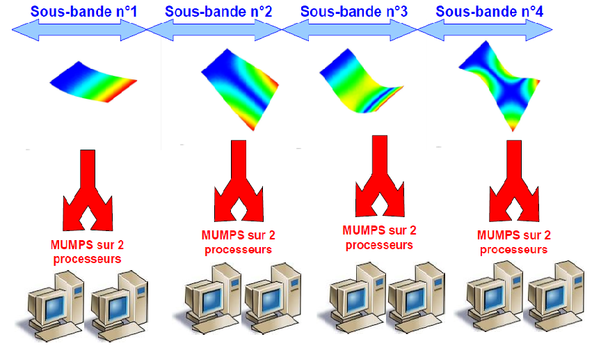
Image 3.14-1- Example of the distribution of calculations of CALC_MODESsur 8 processors with a division into 4 frequency sub-bands

This double level of parallelism (activated by default via with the keyword NIVEAU_PARALLELISME =” COMPLET “) then makes it possible to take full advantage of both aspects.

When you really want to gain peak memory because the calculation does not take place on the machine and you have tried, without success, all the other lever arms [13] _ , you can consciously choose to limit parallelism only at the level of the linear solver [14] _ : NIVEAU_PARALLELISME =” PARTIEL “. This only works with the MUMPS parallel linear solver.

The functional rules are as follows, noting nbproc the number of processors set and nb_sband the number of non-empty sub-bands (=nb_freq-1):

• With NIVEAU_PARALLELISME =” COMPLET “(default) : very big gain in time/improvement or average deterioration of the memory peak RAM.

Image 3.14-2- Scope of use with NIVEAU_PARALLELISME =” COMPLET “.

• With NIVEAU_PARALLELISME =” PARTIEL “:moderate gain in time/significant gain on the memory peak RAM.

Image 3.14-3- Scope of use with NIVEAU_PARALLELISME =” PARTIEL “.

For optimal use of parallelism, it is therefore recommended to:

• Build relatively balanced computing sub-bands. To do this, we can therefore, beforehand, calibrate the spectrum studied*via* one or more calls to INFO_MODE [U4.52.01]. If possible in parallel mode. Then start the parallel calculation CALC_MODES according to the number of sub-bands chosen and the number of processors available.

• To take sub-bands that are finer than sequential, between 10 and 20 modes instead of 40 to 80 modes sequentially. The quality of the modes and the robustness of the calculation will be increased. The memory peak will be reduced as a result. However, you must have enough processors available (and with enough memory).

• Select a number of processors that is a multiple of the number of sub-bands (not empty). In this way, load imbalances that affect performance are reduced.

To reduce the memory peak of a calculation, several lever arms are available: reduce the size of the sub-bands, use the linear solver MUMPS (possibly in OUT_OF_CORE [U4.50.01]) and/or parallelize only this calculation brick (NIVEAU_PARALLELISME =” PARTIEL “).

To effectively use CALC_MODES in parallel, it is therefore proposed to proceed in three steps:

• Modal pre-calibrations prerequisites via INFO_MODE. If possible, in parallel mode (Potential gains in x70 time on hundreds of processors. Memory peak gain RAM up to x2).

• Examine the results produced and break the calculation down into subbands that are modest in size (e.g. 20 modes) and balanced, based on the number of processors available.

• Start the CALC_MODESparallèle calculation itself in POURSUITE mode.

perf016a test case (N=4.0M, 50 modes) splitting into 8 sub-bands	Time elapsed	Memory peak RAM
1 processor	5524s	9Go
8 processors	1002s	5Go
32 processors	643s	4Go
division into 4 sub-bands
1 processor	3569s	2Go
4 processors	1121s	5Go
16 processors	663s	9Go

Table 3.14-1 - Results of CALC_MODES parallel with the default settings (+* *SOLVEUR = MUMPS* *en* *IN_CORE* *and* * **and* *RENUM =” QAMD “) on the test case* **PERF016A. Obtained with Code_Aster v11.3.11 on machine IVANOE (1 or 2 MPI processes by*node) *.**

Seismic study (N=0.7M, 450 modes) splitting into 20 sub-bands	Time elapsed	Memory peak RAM
1 processor	5200s	5Go
20 processors	407s	1Go
80 processors	270s	4Go
division into 5 sub-bands
1 processor	4660s	2Go
5 processors	1097s	8Go
20 processors	925s	5Go

Table 3.14-2 - Results of* *CALC_MODES* **parallel with the default settings (+* *SOLVEUR = MUMPS* *en* *IN_CORE* *and* * **and* ** RENUM =” QAMD “) on a seismic study. Obtained with Code_Aster v11.3.11 on machine IVANOE (1 or 2 MPI processes per node) *.**

Notes:

• In mode NIVEAU_PARALLELISME =” COMPLET “, if the number of processors is not a step multiple of the number of sub-bands (not empty), the remainder of processors is distributed by giving priority to the first sub-bands. A message alerts the user to the potential load imbalance and the suboptimal nature of the calculation.

• In mode NIVEAU_PARALLELISME =” COMPLET “, we deactivated the parallelism of elementary calculations and assemblies that can take place in NORM_MODE. Their cost is marginal anyway.

This deactivation is temporary and just limited to CALC_MODES .However, if the parallel distribution of the data, generated before the CALC_MODES (via AFFE_MODELE/MODI_MODELE), was produced with parameters other than the default values (activation of the keywords * .). DISTRIBUTION CHARGE_PROC0_MAou NB_SOUS_DOMAINE PARTITIONNEUR CHARGE_PROC0_SD) and if you want to find exactly the same distribution, you have to make an explicit call to* MODI_MODELEà after the CALC_MODES.

If this is not done, the parallel partitioning that will follow the CALC_MODES will resume the values by default. This is often the best scenario.

• In mode NIVEAU_PARALLELISME =” COMPLET “, we communicate all the exhumed eigenvectors at the end of CALC_MODES. So the distinction [15] _

between values STURM =” LOCAL “or “GLOBAL “is no longer functionally appropriate. This is not a big deal because the preferred by default mode is the “GLOBAL” mode .

For the practical implementation of parallelism, refer to the generic document [U2.08.06] on parallelism, and to the dedicated paragraph in [U2.06.01] on modal calculation.

3.15. Keyword AMELIORATION

◊ AMELIORATION = /' NON '[DEFAUT]

/” OUI “

Keyword that automatically improves the quality of the calculated modes: mainly modal deformations (which results in a reduction in the error norm) and eigenvalues. This improvement is achieved by a combination of two modal calculations: a first, preferably carried out by a method of simultaneous iterations (keyword OPTION =” BANDE “or” PLUS_PETITE “or” CENTRE “or” TOUT “); the second is carried out transparently for the user, with the method of inverse iterations (OPTION =” PROCHE”) with as enter the eigenvalues estimated using the first calculation.

Remarks :

• The quality of the modes is generally already sufficient after an initial calculation. This option, despite its cost, can however prove to be very interesting for complicated models.

• When this improvement option is activated, the post-verification tests, normally carried out at the end of the first stage (depending on the setting VERI_MODE), are only performed here at the end of the second.

3.16. Keywords for post-processing: NORM_MODE, FILTRE_MODE, IMPRESSION

The NORM_MODE keyword is available for all result types, but the other two are only available for the case of natural vibration modes (TYPE_RESU =” DYNAMIQUE “) and on a physical basis, with real matrices (input matrices of the matr_asse_depl_r type).

3.16.1. Keyword factor NORM_MODE

Used to define the arguments for the normalization of modes. All modes are standardized the same way. The arguments are the same as for the NORM_MODE [U4.52.11] command.

3.16.2. Keyword factor FILTRE_MODE

If present, this keyword is used to introduce mode filtering arguments according to a given criterion. The keywords SEUIL and CRIT_EXTR are the same as for the EXTR_MODE [U4.52.12] command.

3.16.3. Keyword IMPRESSION

Allows you to optionally display the accumulation of values of a chosen modal parameter. The internal keywords CUMUL and CRIT_EXTR have the same meaning as in the EXTR_MODE [U4.52.12] command.

The modal parameter mentioned by CRIT_EXTR ** may not be the same as the one that was possibly used to filter with FILTRE_MODEles calculated modes.

The keyword TOUT_PARApermet to display, after possible normalization, the value of all the modal parameters contained in the data structure produced (frequency, effective masses,…), cf. [R5.01.03]. So we will get in mode_meca_* or mode_gene:

• MASS_GENE, RIGI_GENE

• MASS_EFFE_DX, MASS_EFFE_DY, MASS_EFFE_DZ,

• MASS_EFFE_UN_DX, MASS_EFFE_UN_DY, MASS_EFFE_UN_DZ (compared to the total mass trained),

• FACT_PARTICI_DX, FACT_PARTICI_DY, FACT_PARTICI_DZ.

3.17. Operand INFO

◊ INFO =/1 [DEFAUT]

/2

Indicates the print level in file MESSAGE.

1:	Impression on the file “MESSAGE” of the eigenvalues, their modal position, the reduced damping (if applicable), the error norm a posteriori and some parameters useful to follow the calculation process.
2:	Printing rather reserved for developers.

Table 3.17-1 - Functioning of the keyword INFO depending on its value.

3.18. Operand TITRE

◊ TITRE =ti

Title attached to the concept produced by this operator [U4.03.01].

[1]

If the least-filled sub-band contains only 20 modes, the most supplied sub-band should ideally contain no more than 60 modes. This makes it possible to optimize the calculation costs, the robustness as well as the quality of the modes obtained.

[2]

For reasons of calculation costs, it is better to limit the list to a dozen values. Even if it means relaunching several successive CALC_MODES to scan all the sub-bands you are looking for.

[3]

The sorting criterion is relative, except when the limit sought is close to zero. It then becomes an absolute criterion.

[4]

versus BORNE_MIN/MAX_EFFECT.

[5]

The sorting criterion is relative, except when the limit sought is close to zero. It then becomes an absolute criterion.

[6]

versus BORNE_MIN/MAX_EFFECT.

[7]

Value set via the NPREC parameter of the SOLVEUR keyword (by default ndeci=8).

[8]

In order to minimize the time cost of the (sequential) analysis phase of MUMPS. However, this configuration is done at the expense of memory consumption. But this additional cost is quickly offset by the distribution of data on the processors that parallelism implies.

[9]

Cf. Example of §.

[10]

These tests are expressed in the context of the « work problem » provided for each sub-band to the modal solver. Often this transformed problem is different from the initial problem. The good convergence of this stage therefore does not 100% guarantee that of the initial problem.

[11]

Close to expensive eigenvector communications.

[12]

Because of the MPI buffers required by eigenvector communications at the end of CALC_MODES.

[13]

Cut into more sub-bands, use the modal solver SORENSEN, reduce the size of the projection space via COEF_DIM_ESPACE, use the linear solver MUMPS in OUT_OF_CORE and/or with METIS…

[14]

It’s this type of parallelism that’s deployed in the rest of the code.

[15]

The distinction between the two modes is just computer science here: in the case “GLOBAL”, the Sturm test is implemented at the level of the macro file PYTHON, while in the case “LOCAL”, it is operated in the Fortran sources of the operator (invisible to the user) carrying out the modal calculation by the method of simultaneous iterations.