9. Other loads#
9.1. Keyword LIAISON_INTERF#
LIAISON_INTERF = _F (
           ◆ MACR_ELEM_DYNA = macr_elem_dyna,
           ◇ TYPE_LIAISON =/"RIGIDE" (by default),
                            /"SOUPLE ",
)
The keyword factor LIAISON_INTERF makes it possible to define linear relationships between the physical degrees of freedom of the interfaces of the finite element model part and the generalized coordinates of reduced modes of representation of the interface movements contained in certain macro-elements of static condensation. It can be used with a model containing both finite elements and static macroelements condensing certain sub-domains.
◆ MACR_ELEM_DYNA
Name of the macr_elem_dyna that is used to define the linear relationships between the physical degrees of freedom of the interface between the non-condensed domain modeled in finite elements and a domain condensed by the macroelement and the components of the nodes assimilated to generalized coordinates of interface movement modes. This is only necessary when the interface movement modes are a reduced basis of all constrained modes, each corresponding to a mode of movement for each degree of physical freedom of the interface. Type LIAISON_DDL relationships are thus generated whose coefficients are calculated transparently for the user between the nodes of the dynamic interface of the macro-element and those associated with the reduction base that was used to constitute the macro-element.
◇ TYPE_LIAISON = 'RIGIDE'/'SOUPLE'
If “RIGIDE”, we write the relationship between the physical degrees of freedom of the interface \({U}_{\Sigma }\) and the components of the nodes assimilated to generalized coordinates \(q\) of interface movement modes \(\Phi\) in the form of a simple product: \({U}_{\Sigma }\mathrm{=}{\Phi }_{q}\). This choice makes it possible to have a more rigid connection than by taking into account all the constrained modes each corresponding to a mode of movement for each degree of physical freedom of the interface.
If “SOUPLE”, we write the relationship between the physical degrees of freedom of the interface \({U}_{\Sigma }\) and the components of the nodes assimilated to generalized coordinates \(q\) of interface movement modes \(\Phi\) in the form of a double product: \({\Phi }^{T}{U}_{\Sigma }\mathrm{=}{\Phi }^{T}\Phi q\). This choice makes it possible to have a more flexible connection than by taking into account all the constrained modes each corresponding to a mode of movement for each degree of physical freedom of the interface.
9.2. Keyword RELA_CINE_BP#
RELA_CINE_BP = _F (
   ◆ CABLE_BP = cabl_precont,
   ◇ RELA_CINE =/"OUI" (by default),
                 /"NON ",
   # If: equal_to (" RELA_CINE ", 'OUI')
       ◇ SIGM_BPEL =/"OUI ",
                     /"NON" (by default),
   # If: equal_to (" RELA_CINE ", 'NON')
       ◇ SIGM_BPEL = "OUI ",
   ◇ TYPE_EPX =/"ADHE" (by default),
                /"GLIS ",
                /"FROT ",
   ◇ DIST_MIN = float,
)
This type of load can be defined for a mechanical system comprising a concrete structure and its prestress cables. The initial tension profiles in the cables, as well as the coefficients of the kinematic relationships between the degrees of freedom of the cable nodes and the degrees of freedom of the nodes of the concrete structure are determined beforehand by the operator DEFI_CABLE_BP [U4.42.04]. The cabl_precont concepts produced by this operator provide all the information needed to define the load.
Multiple occurrences are authorized for the keyword factor RELA_CINE_BP, in order to allow in the same call to the operator AFFE_CHAR_MECA to define the contributions of each of the groups of cables that were the subject of separate calls to the operator DEFI_CABLE_BP [U4.42.04]. Each group of cables considered, defined by a cabl_precont concept, is associated with an occurrence of the keyword factor RELA_CINE_BP.
The load thus defined is then used to calculate the equilibrium state of the concrete structure/prestress cables assembly. However, taking this type of load into account is not effective in all resolution operators. For the moment, RELA_CINE_BP loading is only recognized by the STAT_NON_LINE [U4.51.03] operator, exclusively incremental behaviors.
◆ CABLE_BP
Cabl_precont type concept produced by operator DEFI_CABLE_BP [U4.42.04]. This concept provides on the one hand the map of the initial constraints in the elements of the cables in the same group, and on the other hand the lists of kinematic relationships between the degrees of freedom of the nodes of these cables and the degrees of freedom of the nodes of the concrete structure.
◇ SIGM_BPEL = 'OUI'/'NON'
A text-type indicator that specifies the consideration of initial constraints in cables; the default value is” NON “.
In the case “NON”, only the kinematic connection is taken into account. It is useful if you are chaining STAT_NON_LINE while you have pretension cables. For the first STAT_NON_LINE you must have set “OUI”, so that you set up the tension in the cables. On the other hand, for the following STAT_NON_LINE, only kinematic links should be considered as loading and therefore defining the load with SIGM_BPEL = “NON”, otherwise the voltage is counted twice.
Since the restoration of the macro to tension the cables, the user should no longer need to do a AFFE_CHAR_MECA with SIGM_BPEL = “OUI”, this should thus avoid the risk of error.
◇ RELA_CINE = 'OUI'/'NON'
A text-type indicator that specifies the consideration of kinematic relationships between the degrees of freedom of cable nodes and the degrees of freedom of the nodes of the concrete structure; value by default “OUI “.
◇ DIST_MIN = float
See LIAISON_SOLIDE § 5.16.
◇ TYPE_EPX = 'ADHE'/'GLIS'/'FROT'
This keyword only has an effect in CALC_EUROPLEXUS. It allows you to indicate whether you want total cable-concrete connections (i.e. in the 3 directions of space, corresponding to this Aster load), sliding or rubbing connections.
9.3. Keyword VITE_FACE#
VITE_FACE = _F (
           ◇ GROUP_MA = Grma,
           ◆/VNOR = float,
             /DIRECTION = float,
           # If: exists (" DIRECTION ")
               ◆ VITE = float,
)
The keyword factor VITE_FACE allows you to apply speeds to a face in the case of modeling 2D_FLUIDE, AXIS_FLUIDE, 3D_FLUIDE or fluid/structure interface elements (*_ FLUI_STRU).
Topological assignment:
◇ GROUP_MA
The load is affected on the meshes, which are necessarily segments in 2D and triangles or quadrangles in 3D.
There are two ways to affect speed:
If we enter VNOR, then the speed (standard VNOR) will be normal to the face on which it is applied (defined by GROUP_MA);
If we enter DIRECTION which gives the direction of the speed then VITE will be the norm of this speed. This method can only be used if a U_PHI formulation has been chosen (keyword in AFFE_MODELE).
The direction and the norm (VNOR or VITE) can be reals or functions.
9.4. Keyword ONDE_PLANE#
ONDE_PLANE =_F (
            ◇ GROUP_MA = Grma,
            ◆ TYPE_ONDE =/"S",
                           /"P",
                           /"SV",
                           /"SH",
            ◆ DIRECTION = (kx, ky, kz),
            ◆ FONC_SIGNAL = f,
            ◇ DEPL_IMPO = fd,
            ◇ COOR_SOURCE = (x0, y0, z0),
            # If: exists (" COOR_SOURCE ")
                ◇ COOR_REFLECHI = (x1, y1, z1),
)
The keyword factor ONDE_PLANE (only one occurrence is allowed) makes it possible to impose a plane wave seismic loading, corresponding to the loads classically encountered during soil-structure interaction calculations using integral equations (see [R4.05.01]). In harmonics, an elastic plane wave is characterized by its direction, its pulsation and its type (wave \(P\) for compression waves, waves \(S\), \(\mathit{SV}\) or \(\mathit{SH}\) for shear waves). In transition, the pulsation data, corresponding to a stationary wave in time, must be replaced by the data of a displacement profile whose propagation over time in the direction of the wave will be taken into account. More precisely, the following are characterized:
A \(P\) wave using the \(u(x,t)=f\left(k\cdot x-{C}_{p}t\right)\) function;
A \(S\) wave using the \(u(x,t)=f\left(k\cdot x-{C}_{s}t\right)\wedge k\) function;
With:
\(k\) the unit direction vector;
\(f\) the wave profile given in the \(k\) direction;
There can only be one occurrence of this keyword in AFFE_CHAR_MECA * . *
Topological assignment:
◇ GROUP_MA
The load is affected on the absorbent border meshes concerned by the introduction of the incident wave. If nothing is given, by default, all the meshes of modeling ABSO are concerned.
◇ COOR_SOURCE
This list of real parameters makes it possible to determine the phase difference in time due to the passage of the wave, by indicating the coordinates of the entry point \({\mathrm{x}}_{0}\) of plane wave loading into the structure. If this parameter is not present, then operand FONC_SIGNAL will be filled in with a layer of time signals.
◇ COOR_REFLECHI
This list of real parameters allows the reflected wave to be taken into account, activated if the coordinates of the output point \({\mathrm{x}}_{1}\) are given. In this case, the expression of the wave profile taking into account the spatial phase shift associated with the passage of wave \(\dot{f}\left(\mathrm{k}\text{.}(\mathrm{x}-{\mathrm{x}}_{0})-{C}_{m}t\right)\) then becomes \(\dot{f}\left(\mathrm{k}\text{.}(\mathrm{x}-{\mathrm{x}}_{0})-{C}_{m}t\right)+\dot{f}\left(\mathrm{k}\text{.}(2{\mathrm{x}}_{1}-{\mathrm{x}}_{0}-\mathrm{x})-{C}_{m}t\right)\) with \(m\mathrm{=}S\) or \(P\).
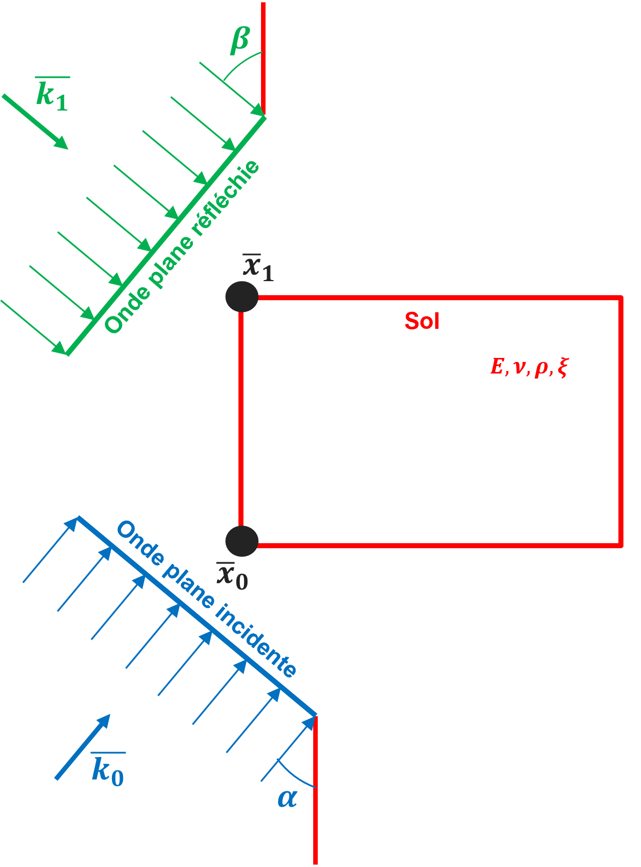
Figure 9.4-1: Diagram of an inclined plane wave propagation in a 2D model
To clarify the use of operands COOR_SOURCE and COOR_REFLECHI we refer to the schema in the. If we consider a plane wave inclined at an angle \(\alpha\) with the vertical, we obviously identify the first point that comes into contact with the field of study, that is to say the point \({\mathrm{x}}_{0}\). This point is considered to be the source point of the incident wave and its coordinates represent the input data for operand COOR_SOURCE. With the same reasoning, if we want to add the consideration of the reflected wave, we can clearly identify the first point on the free surface that generates the reflected wave, that is to say point \({\mathrm{x}}_{1}\). This point is considered to be the source point of the reflected wave and its coordinates represent the input data for operand COOR_REFLECHI.
Notes on using COOR_SOURCE and COOR_REFLECHI operands:
In the case of 2D modeling (D_PLAN, for example) we work in the XY coordinate system. In this case it will be necessary to simply enter the X and Y coordinates of the source point of the incident wave (COOR_SOURCE) and, possibly, of the reflected wave (COOR_REFLECHI). The third coordinate, even if returned, will not be considered;
In the case of vertical propagation, the phase shift of the wave is independent of the X and Y coordinates in 3D (X in 2D). In fact, the wave front is perfectly horizontal and it is out of phase exclusively with respect to the vertical coast (Z in 3D and Y in 2D). Therefore, you can enter any X and Y coordinate in 3D (X in 2D) for the source points of the incident wave and the reflected wave. What matters is to correctly enter the Z coordinate in 3D (Y in 2D) to correctly calculate the phase difference associated with vertical propagation.
◆ TYPE_ONDE = 'P'/'S'/'SV'/'SH'
Type of wave (compression or shear).
\(P\) |
compression wave |
\(\mathit{SV}\) |
shear wave (only in 3D) |
\(\mathit{SH}\) |
shear wave (only in 3D) |
\(S\) |
shear wave (2D only) |
The directions of the waves \(P\), \(\mathit{SV}\) and \(\mathit{SH}\) are determined from the vector \(V\) filled in by DIRECTION. Namely:
\(P\) is collinear to \(V\) and normed to 1,
\(\mathit{SH}\) is the intersection of the horizontal plane and the plane normal to \(V\), and normalized to 1,
\(\mathit{SV}\) is the vector product of \(\mathit{SH}\) and \(P\). There is a case of indeterminacy with this rule when the horizontal plane and the normal plane are confused. In this case, if \(V\) = \(Z\) is purely vertical, we impose \(\mathit{SH}\) = \(Y\), and \(\mathit{SV}\) = \(X\).
◆ DIRECTION
Direction of propagation of the wave.
◆ FONC_SIGNAL
Derived from the \(f(t)\) wave profile for \(t\in [0,\text{+}\mathrm{\infty }[\). Attention: this is the function corresponding to speed \(v(t)=\dot{u}(t)\) that the user gives in FONC_SIGNAL. If the operand COOR_SOURCE is absent, a sheet of speed time signals parameterized by propagation coordinate values \(\mathrm{k}\mathrm{.}\mathrm{x}\) for the variable \(X\) is given.
◇ DEPL_IMPO
Wave profile \(\mathit{fd}(t)\) for \(t\mathrm{\in }\mathrm{[}\mathrm{0,}\text{+}\mathrm{\infty }\mathrm{[}\). Attention: this is the function corresponding to the speed integral \(v(t)=\dot{u}(t)\) that the user obligatory gives in DEPL_IMPO. This optional data is only activated if there are stiffness values added to the absorbing border, activated by the data with a non-zero value of the LONG_CARA operand of the ELAS keyword from DEFI_MATERIAU. If the operand COOR_SOURCE is absent, a sheet of moving time signals parameterized by values of propagation coordinates \(\mathrm{k}\mathrm{.}\mathrm{x}\) for the variable \(X\) is given.
Note regarding the use of this charge: It is strongly recommended to use the keywords ORIE_PEAU_2D or ORIE_PEAU_3D of MODI_MAILLAGE to direct the skin elements affected by absorbent border modeling to outside the domain they delimit.
9.5. Keyword ONDE_FLUI#
ONDE_FLUI = _F (
           ◇ GROUP_MA = Grma,
           ◆ PRES = float,
)
The keyword factor ONDE_FLUI makes it possible to apply a sine wave pressure amplitude normally arriving at a face to models 3D_FLUIDE, 2D_FLUIDE and AXIS_FLUIDE.
Topological assignment:
◇ GROUP_MA
The wave is applied to these meshes. They are necessarily edge meshes (segments in 2D and triangles/quadrangles in 3D).
◆ PRES
Pressure amplitude of sine wave incident waves arriving normally at the face.
9.6. Keyword FLUX_THM_REP#
FLUX_THM_REP = _F (
           ◆/TOUT = "OUI" (or not specified),
             /GROUP_MA = grma,
           ◆ | FLUN = float,
             | FLUN_HYDR1 = float,
             | FLUN_HYDR2 = float,
             | FLUN_FRAC = function/formula/table cloth,

)
The keyword factor FLUX_THM_REP makes it possible to apply a heat flow and/or a fluid mass supply (hydraulic flow) to a 2D or 3D continuous medium domain. Hydraulic flows (water and steam) are defined by:
With the density of water \({\mathrm{\rho }}_{e}\), the density of steam \({\mathrm{\rho }}_{\mathrm{\nu }}\), the density of steam, the pressure of water \({P}_{e}\) (degree of freedom PRE1), and the pressure of steam \({P}_{v}\) (degree of freedom PRE2).
Heat flow is defined by:
With the mass enthalpies of water \({h}_{m}^{l}\), steam \({h}_{m}^{v}\), air \({h}_{m}^{a}\), and air flow \({\mathrm{\varphi }}^{a}\).
Topological assignment:
◆/TOUT = "OUI" (or not specified),
  /GROUP_MA = grma,
The load is affected on these meshes They are necessarily edge meshes (segments in 2D and triangles/quadrangles in 3D). This load can only be used in (thermo) -hydraulics or in pure hydraulics (THM, THH,,, THHM, HMou HHM).
◆ | FLUN
Heat flow value.
◆ | FLUN_HYDR1
Value of the hydraulic flow associated with the water component.
◆ | FLUN_HYDR2
Value of the hydraulic flow associated with the steam component.
◆ | FLUN_FRAC
Value of hydraulic flow injected into a cohesive interface for HM- XFEM models. This loading is imposed exclusively using a space function on the main elements and not on the edge elements. For more details on the use of this keyword, refer to the [R7.02.18] and [U2.05.02] documentation.
9.7. Keyword ECHANGE_THM#
ECHANGE_THM = _F (
           ◆/TOUT = "OUI" (or not specified),
             /GROUP_MA = grma,
           ◆ COEF_11 = float,
           ◇ COEF_12 = float,
           ◇ COEF_21 = float,
           ◇ COEF_22 = float,
           ◆ PRE1_EXT = float,
           ◇ PRE2_EXT = float,
)
The keyword factor ECHANGE_THM allows for an unsaturated modeling to apply to a 2D or 3D continuous medium domain an exchange condition on external hydraulic pressures. The resulting hydraulic flows (water and air) are defined by:
With capillary pressure \({p}_{1}\) (degree of freedom PRE1) and gas pressure \({p}_{2}\) (degree of freedom PRE2). \({M}_{w}+{M}_{\text{vp}}\) corresponds to water flow (sum of liquid water flow \({M}_{w}\) and steam flow \({M}_{\text{vp}}\)) and \({M}_{\text{ad}}+{M}_{\text{as}}\) corresponds to air flow (sum of dissolved air flow \({M}_{\mathit{ad}}\) and dry air flow \({M}_{\text{as}}\)).
Topological assignment:
◆/TOUT = "OUI" (or not specified),
  /GROUP_MA = grma,
The load is affected on these cells They are necessarily edge meshes (segments in 2D and triangles/quadrangles in 3D). This loading can only be used for unsaturated models such as THH2MS, THH2S,, HH2MSou HH2S.
◆ PRE1_EXT
Value of external capillary pressure.
◇ PRE2_EXT
External gas pressure value (0 by default).
◆ COEF_11
exchange coefficient C11 (cf. eq.) relating the flow of water to the capillary pressure.
◇ COEF_12
exchange coefficient C12 (cf. eq.) linking the water flow to the gas pressure (0 by default).
◇ COEF_21
exchange coefficient C21 (cf. eq.) connecting the air flow to the capillary pressure (0 by default).
◇ COEF_22
exchange coefficient C22 (cf. eq.) connecting the air flow to the gas pressure (0 by default).
9.8. Keyword ECHANGE_THM_HR#
ECHANGE_THM_HR = _F (
           ◆/TOUT = "OUI" (or not specified),
             /GROUP_MA = grma,
           ◆ HR_EXT = float,
           ◆ ALPHA = float,
           ◆ PVAP_SAT = float,

)
The keyword factor ECHANGE_THM_HR allows for unsaturated modeling to apply to a 2D or 3D continuous medium domain a mixed vapour density exchange condition (proportional to relative humidity). The flow of water is then written as:
with \(\rho_{vp}\) the vapor density.
Knowing that the relative humidity RH is a function of the density via the saturation vapor density \(\rho_{vp}^{sat}\):
The flow is then expressed
We can express this equation as a function of the capillary pressure (Pc which is an unknown of the model) thanks to the Kelvin relationship that is:
with \({M}_{H2O}\) the molar mass of water, R the ideal gas constant, and T the temperature. In the end, the expression of flow becomes:
Topological assignment:
◆/TOUT = "OUI" (or not specified),
  /GROUP_MA = grma,
◆ HR_EXT
Relative humidity outside.
◆ ALPHA
Exchange coefficient
◆ PVAP_SAT
Saturating vapour pressure
9.9. Keyword FORCE_SOL#
FORCE_SOL = _F (
           ◆/GROUP_NO_INTERF = grno,
             /SUPER_MAILLE = my,
           ◆ | UNITE_RESU_MASS = unit,
             | UNITE_RESU_RIGI = unit,
             | UNITE_RESU_AMOR = unit,
           ◇ UNITE_RESU_FORC = unit,
           ◇ NB_PAS_TRONCATURE = int,
           ◇ TYPE =/"BINAIRE ",
                    /"ASCII" (by default),
)
The keyword factor FORCE_SOL makes it possible to take into account the internal force of a ground domain by using the temporal evolutions of the contributions in stiffness, mass and damping of the ground impedance. The ground impedance extracted at the initial instant makes it possible to constitute by MACR_ELEM_DYNA a macroelement representing the behavior of the ground domain that is added to the structure model. The dynamic interface of the macro-element is described either by a supermesh of the model containing both the structure and this macro-element, or by a group of nodes if the physical interface coincides with the modal dynamic interface.
It is also possible to take into account, if it exists, the temporal evolution of seismic forces, assigned to this same dynamic interface in the form of a logical unit.
This type of load is taken into account in command DYNA_NON_LINE. An example of use is provided in test case MISS03B [V1.10.122].
There can only be one occurrence of this keyword in AFFE_CHAR_MECA * . *
Topological assignment:
◆/GROUP_NO_INTERF = grno,
  /SUPER_MAILLE = my,
These operands make it possible to describe the dynamic interface of the macroelement representing the behavior of the soil domain that is added to the structure model either by a supermesh of the model containing both the structure and this macroelement by the keyword SUPER_MAILLE, or by a group of nodes by the keyword GROUP_NO_INTERF, or by a group of nodes by the keyword if the physical interface coincides with the modal dynamic interface.
◆ | UNITE_RESU_MASS = unit,
  | UNITE_RESU_RIGI = unit,
  | UNITE_RESU_AMOR = unit,
These operands make it possible to introduce the temporal evolutions of the contributions in stiffness, mass and damping of the ground impedance in the form of logic units.
◇ TYPE =/"BINAIRE ",
         /"ASCII" (by default)
This operand makes it possible to introduce the common writing format (“ASCII” or “BINAIRE”) of the temporal evolutions of the contributions in stiffness, mass and damping of the ground impedance entered in the form of logical units by the previous operands UNITE_RESU_ *. The operand value must be consistent with the value entered in operand TYPE_FICHIER_TEMPS when calculating the option TYPE_RESU =” FICHIER_TEMPS “by CALC_MISS.
◇ UNITE_RESU_FORC
This operand makes it possible to introduce, if it exists and in the form of a logical unit, the temporal evolution of seismic forces, assigned to the dynamic interface of the macro-element representing the behavior of the ground domain that is added to the structure model.
◇ NB_PAS_TRONCATURE = int,
This operand makes it possible to introduce (if present) a truncation of the calculation of the contribution to the second member of the ground force in DYNA_NON_LINE. This truncation takes place on the basis of the displacement fields stored at the preceding moments. Following tests, we realize that it is often enough to truncate the sum over the last 50 to 100 steps of time instead of making the full sum over all the previous stored moments, which is the default option. It is therefore advisable to use as a practical value the integer value of the maximum between 50 and a tenth of the total number of stored time steps.