4. Keyword factor MAZARS#
The Mazars behavior model is a model of damaging elastic behavior used to describe the softening behavior of concrete. It distinguishes between traction and compression behavior.
4.1. Operand CODIFICATION#
The defi_mater_gc command can use best practices or advice from codifications to determine the parameters of the MAZARS behavior law.
♦ CODIFICATION = “BAEL91”|”EC2”|”TEST”
“BAEL91”: indicates that the parameters used in the definition of materials come from codification BAEL1991.
“EC2”: indicates that the parameters used in the definition of materials come from codification EUROCODE2.
“ESSAI “:indicates that the parameters used in the definition of materials come from test.
For example, according to BAEL 1991, for the concrete material knowing its characteristic compressive strength fcj, its tensile strength can be estimated by: \(\mathit{FTJ}=0.6+0.06\mathit{FCJ}\) where FTJ and FCJ are in \(\mathit{MPa}\).
4.1.1. Case where CODIFICATION =” BAEL91 “#
The parameters used in the definition of materials come from codification BAEL1991.
♦ unite_ CONTRAINTE
Unit of constraint of the problem [:math: mathit {MPa} |:math: mathit {Pa}]: Mega-Pascal or Pascal. Entering this operand is mandatory, because the formulas used in the following require knowing if the material parameters are en:math: mathit {Pa} or:math: mathit {MPa} or:math: mathit {MPa}. The material parameters that are returned by the command are in the same unit system. UNITE_CONSTRAINT must therefore be compatible with the units of the study.
\(\mathit{Pa}\): the material parameters are homogeneous to \(\mathit{Pa}\).
\(\mathit{MPa}\): the material parameters are homogeneous to \(\mathit{MPa}\).
♦ FCJ
Peak stress in compression, in \(\mathit{Pa}\) or \(\mathit{MPa}\), depending on the value of UNITE_CONTRAINTE.
4.1.2. Case where CODIFICATION =” EC2 “#
♦ unite_ CONTRAINTE
Unit of constraint for the problem \(\mathit{MPa}\) or \(\mathit{Pa}\): Mega-Pascal or Pascal. Entering this operand is mandatory, as it is necessary to return the material parameters to the unit system used to do the study.
♦ CLASSE
The compressive strength of concrete is designated by strength classes linked to the characteristic strength measured on a cylinder or on a cube, in accordance with EN 206-1.
The classes available in the operator are all those defined in EUROCODE 2:
“C12/15” “C16/20” “C20/25” “C20/25” “C25/30” “C30/37” “C35/45” “” C40/50 “
“C45/55” “C50/60” “C55/67” “C55/67” “C60/75” “C70/85” “C80/95” “” C90/105 “
4.1.3. Case where CODIFICATION =” ESSAI “#
In this case, the user must fill in all the characteristics necessary to determine the parameters of the law of behavior of MAZARS. The user must provide these characteristics in a system of units compatible with his study.
Mandatory parameters:
♦ FCJ: Peak stress during compression.
♦ EIJ: Young’s module.
♦ EPSI_C: Peak deformation under compression.
♦ FTJ: Peak stress during traction.
The optional parameters, shown in the table, are those found under the keyword factor MAZARSde in the defi_material command [U4.43.01].
e PSD0 |
Deformation damage threshold |
EPST0 EPSC0 |
Tensile and compression damage threshold. |
ac, BC |
Coefficient for fixing the shape of the post-peak curve under compression. |
at, bT |
Coefficient for fixing the shape of the post-peak curve under traction. |
K |
Shear correction parameter. |
Table 4.1.3-a : Material parameters of law MAZARS.
◊ Nu:Poisson’s ratio.
◊ SIGM_LIM: Boundary constraint.
◊ EPSI_LIM: Boundary deformation.
4.2. Operation#
4.2.1. Parameters of law MAZARS#
The parameters of the law are determined using the following characteristics: FCJ, EIJ, EPSI_C, FTJ. The formulas are:
\({\epsilon }_{0}={f}_{\mathit{tj}}/{E}_{\mathit{ij}}\) \(\beta =1.10\) \({B}_{T}={E}_{\mathit{ij}}/{f}_{\mathit{tj}}\) \({A}_{T}=0.70\)
\({B}_{c}=\frac{1}{{\epsilon }_{c}\nu \sqrt{2}}\) \({A}_{c}=\frac{\left(\frac{{f}_{\mathit{cj}}\mathrm{\nu }\sqrt{2}}{{E}_{\mathit{ij}}}-{\mathrm{\epsilon }}_{0}\right)}{{\mathrm{\epsilon }}_{c}\mathrm{\nu }\sqrt{2}\mathrm{exp}\left({B}_{c}({\mathrm{\epsilon }}_{0}-{\mathrm{\epsilon }}_{c}\mathrm{\nu }\sqrt{2})\right)-{\mathrm{\epsilon }}_{0}}\)
\({\sigma }_{\mathit{ELS}}=0.6{f}_{\mathit{cj}}\) \({\epsilon }_{\mathit{ELU}}=3.5‰\)
\({A}_{c}\) and \({B}_{c}\) are determined by solving the equations from writing \(\mathrm{1D}\) of the behavior of MAZARS in order to respect the stress and deformation at the peak, as well as the horizontal tangent at the peak.
\({B}_{c}\) is achieved by solving \(f\text{'}({\epsilon }_{c})=0\)
\({A}_{c}\) by solving \({f}_{\mathit{cj}}=f({\epsilon }_{c})\).
4.2.2. In the case BAEL 1991#
Two operands are required: unite_containte, FCJ.
The command determines the quantities required using formulas or rules from bael91. In the formulas below the quantities \({f}_{\mathit{cj}},{f}_{\mathit{tj}},{E}_{\mathit{ij}}\) are in \(\mathit{MPa}\).
\({E}_{\mathit{ij}}=11000.0\sqrt[3]{{f}_{\mathit{cj}}}\) \({f}_{\mathit{tj}}=0.6+0.06{f}_{\mathit{cj}}\) \({\epsilon }_{c}=0.620E-3\sqrt[3]{{f}_{\mathit{cj}}}\) \(\nu =0.200\)
The parameters of the law of MAZARSsont were then determined.
4.2.3. In the case EUROCODE 2#
Two operands are required: unite_containte, CLASSE.
The command determines the quantities required by formulas or rules from EUROCODE 2. In the formulas below the quantities \({f}_{\mathit{ck}},{f}_{\mathit{cm}},{f}_{\mathit{ctm}},{E}_{\mathit{cm}}\) are in \(\mathit{MPa.}\)
\({f}_{\mathit{ck}}\): characteristic compression strength measured on a cylinder at 28 days.
\({f}_{\mathit{cm}}\): average compressive strength of concrete at 28 days.
\({f}_{\mathit{cm}}={f}_{\mathit{ck}}+8.0\)
\({f}_{\mathit{ctm}}\): average tensile strength of concrete.
\({f}_{\mathit{ctm}}=\{\begin{array}{cc}0.30{{f}_{\mathit{ck}}}^{2/3}& \mathit{pour}\mathit{classe}\le \text{C50/60}\\ 2.12\mathrm{log}(1+{f}_{\mathit{cm}}/10)& \mathit{pour}\mathit{classe}>\text{C50/60}\end{array}\)
\({E}_{\mathit{cm}}\): tangent module
\({E}_{\mathit{cm}}=22.0E+03{\left(\frac{{f}_{\mathit{cm}}}{10}\right)}^{0.3}\)
\({\epsilon }_{\mathit{c1}}\): deformation at the peak in \(‰\)
\({\epsilon }_{\mathit{c1}}=0.7{{f}_{\mathit{cm}}}^{0.31}\mathit{toujours}\le 2.8\)
\({\epsilon }_{\mathit{cu1}}\): ultimate limit deformation in \(‰\).
\({\epsilon }_{\mathit{cu1}}=\{\begin{array}{cc}2.80+27{\left[\frac{98-{f}_{\mathit{cm}}}{100}\right]}^{4}& \mathit{pour}\mathit{classe}>\text{C50/60}\\ 3.5& \mathit{pour}\mathit{classe}\le \text{C50/60}\end{array}\)
The parameters of the law of MAZARSsont were then determined.
4.2.4. In case ESSAI#
Four operands are required: FCJ, EIJ,, EPSI_C, FTJ. The parameters of the MAZARS law of behavior are determined as before.
If optional operands shown in the table are filled in, they are taken into account by the command. It is therefore necessary to ensure the consistency of the quantities provided, in particular in the following cases:
the user gives \({B}_{c}\). Equation \(f\text{'}({\epsilon }_{c})=0\) may not be verified, in this case the behavior will pass through the point \({f}_{\mathit{cj}}\) but \({f}_{\mathit{cj}},{\epsilon }_{c}\) will no longer be an extremum.
the user gives \({A}_{c}\). Equation \({f}_{\mathit{cj}}=f({\epsilon }_{c})\) may not be true, in which case the behavior will not pass through the point \({f}_{\mathit{cj}}\) and \({\epsilon }_{c}\).
4.3. Example of use#
To define a concrete that has a behavior of MAZARS with a characteristic strength of \(40.0\mathit{MPa}\) for a study whose stresses must be in \(\mathit{Pa}\), the command is used as follows:
BETONM = DEFI_MATER_GC (
MAZARS = _F (FCJ = 40.0E+06, 40.0E+06,, ), ), UNITE_CONTRAINTE
)
The command prints all the values that are used to define the material into the message file.
== Parameters of law MAZARS [Pa] ==
Elasticity part:
E = 3.76194246E+10, NU = 2.00000000E-01,
Non-linear part:
BT = 1.25398082E+04, K = 0.70000000E+00,
AT = 7.00000000E-01, EPSI_LIM = 3.50000000E-03,
BC = 1.66741558E+03, SIGM_LIM = 2.40000000E+07,
AC = 1.28292129E+00, EPSD0 = 7.97460364E-05,
For information:
FCJ = 4.000E+07, FTJ = 3.0000E+06, = 3.0000E+06, EPSI_C = 2.12036757E-03,
The table gives sets of parameters obtained with the rules described above.
\(\mathit{Fcj}\) [\(\mathit{MPa}\)] |
30.0 |
35.0 |
35.0 |
40.0 |
45.0 |
50.0 |
|
\(\mathit{Ftj}\) [\(\mathit{MPa}\)] |
2.4 |
2.7 |
2.7 |
3.0 |
3.3 |
3.6 |
|
\(\mathit{Young}\) [\(\mathit{MPa}\)] |
34180.0 |
35982.0 |
35982.0 |
37619.0 |
39126.0 |
40524.0 |
|
\(\mathit{Nu}\) |
0.2 |
0.2 |
0.2 |
0.2 |
0.2 |
0.2 |
|
\({\mathit{Epsi}}_{c}\) |
1.93E-03 |
2.03E-03 |
2.03E-03 |
2.21E-03 |
2.28E-03 |
2.28E-03 |
|
\(\mathit{At}\) |
0.7 |
0.7 |
0.7 |
0.7 |
0.7 |
0.7 |
|
\(\mathit{Bt}\) |
14241.0 |
13327.0 |
13327.0 |
125 39.8 |
11856.0 |
11257.0 |
|
\(\mathit{Epsid}0\) |
7.02E-05 |
7.50E-05 |
7.9 7 E-05 |
8.43E-05 |
8.88E-05 |
8.88E-05 |
|
\(\mathit{Bc}\) |
1835.2 |
1743.3 |
1743.3 |
1667.4 |
1603.2 |
1547.9 |
|
\(\mathit{Ac}\) |
1.128 |
1.209 |
1.209 |
1.209 |
1.283 |
1.351 |
1.415 |
Table 4.3-a: Parameters for law MAZARS.
The figure shows the various compression curves obtained with the values in the table.
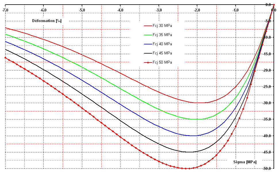
Figure 4.3-a: Law of MAZARS \(\sigma =f(\epsilon )\) compression curves.