4. Operands RELATION = GLRC_DM

The documentation for model GLRC_DM [R7.01.32] will be consulted.

4.1. Keyword BETON

The keyword factor BETON defines the geometric and material characteristics of concrete.

4.1.1. Operand MATER

MATER = mat_concrete

Define the name of the material necessarily produced by DEFI_MATER_GC/BETON_GLRC used for concrete. This operand makes it possible to verify that the parameters associated with the behavior of concrete exist in the material.

4.1.2. Operand EPAIS

EPAIS = ep

Defines the thickness of the concrete plate. We check that \(\mathit{ep}\mathrm{\ge }0\).

Note:

The value of this thickness should be the same as that given in AFFE_CARA_ELEM for shell elements using the mat_beton material (defined by DEFI_GLRC).

4.2. Keyword NAPPE

The keyword factor NAPPE defines the geometric and material characteristics of passive reinforcements. This keyword can only be set once. In fact, under the hypothesis of isotropy in elasticity of the law of behavior GLRC_DM, all the reinforcements are necessarily identical and equidistant from the neutral fiber.

4.2.1. Operand MATER

MATER = mat_steel

Defines the name of the material necessarily produced by DEFI_MATE_GC/ACIER used for passive reinforcements.

This operand makes it possible to recover the material parameters used for passive reinforcements (Young’s modulus \({E}_{a}\), Poisson’s ratio \({\nu }_{a}\) and elastic limit \({\sigma }_{\mathrm{ya}}\)).

4.2.2. Operands OMX and OMY

OMX = Wx

OMY = Wy

Define the steel sections \({\Omega }_{x}\) and \({\Omega }_{y}\) of any of the two given reinforcement beds in the directions \(x\) and \(y\) (in linear \({m}^{2}/m\) if the thickness is given in \(m\)). It should be noted that the formulation of model GLRC_DM requires that the two reinforcement layers be identical.

We check that \({\Omega }_{x}>0\) and \({\Omega }_{x}={\Omega }_{y}\) .With the two layers of reinforcement in the reinforced concrete section, we will therefore have a total reinforcement rate equal to \(2{\Omega }_{x}=2{\Omega }_{y}\).

4.2.3. RX and RY operands

RX = rxx

RY = ry

Define the dimensionless position of a reinforcement bed in relation to the thickness of the concrete shell, given in the directions \(x\) and \(y\) (\(\mathrm{-}1\mathrm{\le }\mathit{rx}\mathrm{\le }1\), \(\mathrm{-}1\mathrm{\le }\mathit{ry}\mathrm{\le }1\),).

We check that \(\mathit{rx}\mathrm{=}\mathit{ry}\).

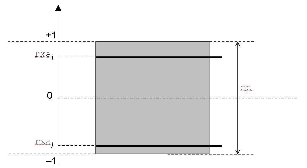
Figure 4.2.3-a : D: D** definition of the dimensioned position of the reinforcement beds.

4.3. Operand RHO

RHO = rho

Optional operand allowing the user to define the equivalent density of the reinforced concrete slab. In the case where the operand is not defined, the density is calculated in the following way:

\({\rho }_{\mathit{eq}}\mathrm{=}{\rho }_{b}+\frac{{\rho }_{a}}{h}({\Omega }_{x}^{\text{sup}}+{\Omega }_{x}^{\text{inf}}+{\Omega }_{y}^{\text{sup}}+{\Omega }_{y}^{\text{inf}})\)

Where \({\rho }_{a}\) designates the density of steel and is recovered in the mat_steel concept provided by the MATER operand of the keyword NAPPE.

Where \({\rho }_{b}\) designates the density of concrete and is recovered in the concept mat_betonprovided by the MATER operand of the keyword BETON.

Where \(h\) is the thickness provided by the EPAIS keyword.

4.4. Operands AMOR_ALPHA, AMOR_BETA, and AMOR_HYST

AMOR_ALPHA = amor_alpha

AMOR_BETA = amor_beta

AMOR_HYST = amor_hyst

Optional operand allowing the user to define the coefficients \(\alpha\) and \(\beta\) that are used to build the Rayleigh damping matrix and \(\eta\) for the hysteretic damping.

\(C=\alpha K+\beta M\)

Refer to the mechanical damping modeling documents [U2.06.03] and [R5.05.04].

If the operands are not specified in the command, they take the values defined in the mat_beton concept provided by the MATER operand of the BETON keyword.

4.5. Keyword factor PENTE

4.5.1. Operand TRACTION

◊ TRACTION =/RIGI_ACIER [DEFAUT]

/PLAS_ACIER /UTIL

The keyword TRACTION defines the method for calculating the post-elastic slope. In fact, it is possible to perform this calculation using three methods called RIGI_ACIER, PLAS_ACIER and UTIL. These three slope calculations make it possible to set up three different calibration methods according to the material properties entered for traction. In the case where the elastic limit of steels is not known, the adjustment methods RIGI_ACIER, i.e. post-elastic slope equal to the steels” stiffness recovery slope, and UTIL, i.e. post-elastic slope cuts the steels stiffness recovery slope at a maximum deformation whose value is imposed by the user, are accessible (this method is not suitable for maximum deformations smaller than the trough of the curve). for reference, see). In the case where the limit of elasticity of steels is known, it is possible to use the method of adjusting to the limit of plasticity of steels (PLAS_ACIER). The various recalibration methods are illustrated by the following figures.

Figure 4.5.1-a: Tensile Curve (GLRC_DM vs Reference) Adjustment PENTE = RIGI_ACIER

Figure 4.5.1-b: Tensile Curve (GLRC_DM vs Reference) Adjustment PENTE = UTIL

Figure 4.5.1-c: Tensile Curve (GLRC_DM vs Reference) Adjustment PENTE = PLAS_ACIER

In the case of the adjustment to the maximum deformation (TRACTION = UTIL), it is necessary to enter the maximum deformation in the membrane (EPSI_MEMB).

4.5.2. Operand FLEXION

◊ FLEXION =/RIGI_INIT [DEFAUT]

/RIGI_ACIER

/PLAS_ACIER

/UTIL

The keyword FLEXION defines the method for calculating the post-elastic slope. In fact, it is possible to perform this calculation using two methods called RIGI_INIT, RIGI_ACIER, PLAS_ACIER and UTIL.

The options RIGI_ACIER and PLAS_ACIER correspond to the settings exposed for flexure in 4.5.1, transposed to the case of flexure.

In the case of option RIGI_INIT, the bilinear approximation of the flexural response of the section is determined in the following way (cf [R7.01.32]):

• the elasticity threshold is fixed for a value M that deviates from the theoretical curve by 5%;

• the second slope is defined so that the bilinear law is tangent to the theoretical curve.

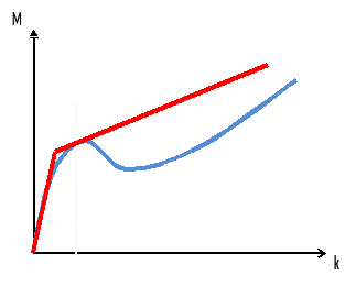
Figure 4.5.2-a: Bending curve (GLRC_DM vs Reference) Setting PENTE = RIGI_INIT

In the case of option UTIL, the bilinear approximation of the flexural response of the section is determined so as to reduce the area relative to the theoretical response of the section up to the curvature kf (KAPPA_FLEX). (see [R7.01.32])

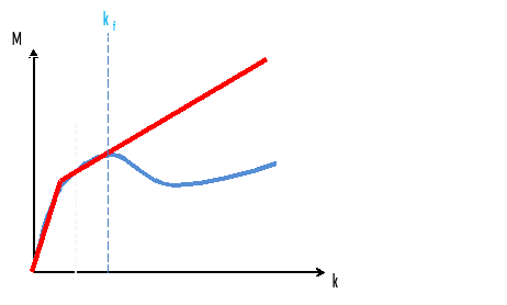
Figure 4.5.2-b: Bending curve (GLRC_DM vs Reference) Setting PENTE = UTIL

4.5.3. Operand EPSI_MEMB

EPSI_MEMB = em

Define the value of the maximum deformation in the membrane in the case TRACTION = UTIL.

4.5.4. Operand KAPPA_FLEX

KAPPA_FLEX = kf

Define the value of the maximum flexural curvature (inverse of a length) in the case FLEXION = UTIL.

4.6. Keyword CISAIL

The simple keyword CISAIL makes it possible to define whether the homogenized elastic parameters are those calculated by homogenization for a standard application of the behavior model (CISAIL = NON) or those calculated for a particular application in order to respect the fact that when one is in flat shear for pure shear the stiffness of the steels does not intervene in the elastic behavior (CISAIL = OUI).

4.7. Keyword INFO

With INFO = 2, we get the Print in RESULTAT format of the list of homogenized parameters used as input to the behavior model GLRC_DM: elasticity, thresholds and damaging behavior.

4.8. Example of use

We can consult the example of use reported in test SSNS106A, in a traction-compression situation, and in test SSNS106B, in an alternating flexure situation, cf. [V6.05.106]. It can be used to verify on the case under study the consequences in terms of response for elementary static loads alternating between the choice of parameters and identification methods.