2. 1D-3D non-intrusive toggle#
A switch from a beam model to a mixed beam-3D model saves considerably in calculation time for an accuracy equivalent to an entire 3D model [bib2].
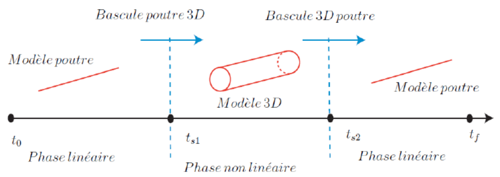
Image 1.1-a weighting functions in the Harlequin frame
Code_Aster allows you to initialize a dynamic calculation with non-zero displacement fields, speeds and accelerations (ETAT_INIT in dynamic calculation operators). These initialization fields can be calculated beforehand and then transformed into a field in*Code_Aster*.
2.1. Theoretical principle of the seesaw#
The switch consists in going from a Beam model (Up is the beam solution of system \({M}_{p}\ddot{{U}_{p}}+{C}_{p}\dot{{U}_{p}}+{K}_{p}{U}_{p}\mathrm{=}{f}_{p}\)) to a 3D model (U3D solution to be initialized) through a relevant initialization of the 3D solution. The basic principle is as follows:
from the Up beam solution, create a 3D solution PUp for the rigid section hypothesis
write the 3D displacement field as being the sum of the extruded field of the Pup Beam type and of a corrective displacement field noted U3Dc, taking into account the deformation of the section :: **
\({U}_{\mathrm{3D}}\mathrm{=}{\mathit{PU}}_{p}+{U}_{\mathrm{3Dc}}\)
The dynamics of the 3D model will then be written as follows:
\({M}_{\mathrm{3D}}(\ddot{{\mathit{PU}}_{p}}+\ddot{{U}_{\mathrm{3Dc}}})+{C}_{\mathrm{3D}}(\dot{{\mathit{PU}}_{p}}+\dot{{U}_{\mathrm{3Dc}}})+{K}_{\mathrm{3D}}({\mathit{PU}}_{p}+{U}_{\mathrm{3Dc}})\mathrm{=}{f}_{\mathrm{3D}}\)
correct the displacements, in static, under the effect of a force vector f 3Dc calculated as follows:
\({f}_{\mathrm{3Dc}}\mathrm{=}{K}_{\mathrm{3D}}{U}_{\mathrm{3Dc}}\mathrm{=}{f}_{\mathrm{3Dc}}(t\mathrm{=}{t}_{b})\mathrm{-}{M}_{\mathrm{3D}}\ddot{{\mathit{PU}}_{p}}\mathrm{-}{C}_{\mathrm{3D}}\dot{{\mathit{PU}}_{p}}\mathrm{-}{K}_{\mathrm{3D}}{\mathit{PU}}_{p}\)
The static correction is carried out over 3 successive time steps: the switching time tbas well as the one before (tb-1 = tb-Δt) and the next one (tb+1 = tb+ Δt) where Δt is the calculation time step. A speed correction is deduced from this, which is written as follows:
\(\dot{{U}_{\mathrm{3D}}}\mathrm{=}\frac{{\left[{\mathit{PU}}_{p}+{U}_{\mathrm{3Dc}}\right]}_{({t}_{b+1})}\mathrm{-}{\left[{\mathit{PU}}_{p}+{U}_{\mathrm{3Dc}}\right]}_{({t}_{b\mathrm{-}1})}}{2\Delta t}\) (Centered Finite Differences)
The accelerations, for their part, are either calculated in the same way according to a Centered Finite Differences scheme,
\(\ddot{{U}_{\mathrm{3D}}}\mathrm{=}\frac{{\left[{\mathit{PU}}_{p}+{U}_{\mathrm{3Dc}}\right]}_{({t}_{b\mathrm{-}1})}+{\left[{\mathit{PU}}_{p}+{U}_{\mathrm{3Dc}}\right]}_{({t}_{b+1})}\mathrm{-}2{\left[{\mathit{PU}}_{p}+{U}_{\mathrm{3Dc}}\right]}_{({t}_{b})}}{{\Delta t}^{2}}\)
be determined automatically by Code_Aster in the case of the use of an implicit time integration scheme.
The correction includes a correction of the arrow as well as a correction to take into account the deformation of the section.
2.2. Example of implementation#
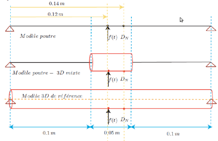
The methodology is explained below for a double-supported beam problem subjected to dynamic sinusoidal excitation for 3s.
The simulation starts with a beam model. The dynamic calculation on the single-beam model takes place from the initial instant t0 until the moment of switching to the 3D model (here, t0=0s, tb=2.4s).
Ti=0;
Qf=3.0;
Tb=2.4;
dt=0.0015;
tb_1=tb-dt;
TB_2=tb+dt;
The following operations will be used for the switch.
# Creating the empty Python mesh
mail_py = MAIL_PY ()
# Converting an Aster mesh to a Python mesh
mail_py.fromaster (“Mail”)
# Node coordinates
COORD_3D = mail_py.cn
ipouAllNode = mail_py.gno.get (“allNode”)
IPou RP1 = mail_py.gno.get (“RP1”)
IPou RP2 = mail_py.gno.get (“RP2”)
C3Z = zeros ((len (COORD_3D) ,1))
For i in range (len (C3DZ)):
C3DZ [i] = COORD_3D [i] [2]
C1 DZ1 = []
min=1112
While (min! =111):
i = 0
s = int ((abs (C3DZ [i]) +adjust) *Pow) /float (Pow)
For i in range (len (C3DZ)):
if (int ((C3DZ [i] +adjust) *Pow) /float (Pow)) ==min:
C3DZ [i] = 1111
elif ((int ((C3DZ [i] +adjust) *Pow) /float (Pow)) < s):
s = int ((C3DZ [i] +adjust) *Pow) /float (Pow)
If (min! =s):
Min=s
C1 DZ1 .append (min)
C1D = zeros ((len (C1 DZ1) -1.3))
For i in range (len (C1D)):
C1D [i] [0] = 0
C1D [i] [1] = 0
C1D [i] [2] = C1 DZ1 [i]
# Function to find the section that corresponds to a z value
def orderSect (s):
jk=0
while (C1D [jk] [2]! =z):
jk=jk+1
Return JK
At the switching time tb, the displacements Up, the speeds Vp and the accelerations Ap of the neutral fiber of the beam are recovered by the operator CREA_CHAMP, operation “EXTR”. Then, the components (DX, DY, DZ, DRX, DRY, DRZ) are extracted into Python tables.
Time = np.Array ([Tb,Tb_1,Tb_2])
nbpas = time.shape [0]
U0= []
U1= []
U2= []
For i in range (nbpas):
step = time [i]
DEP = CREA_CHAMP (OPERATION =” EXTR “,
TYPE_CHAM =” NOEU_DEPL_R “,
RESULTAT = DLT,
NOM_CHAM =” DEPL “,
INST =not,);
Upx = DEP. EXTR_COMP (“DX”, [“allNode”]) .values;
Upy = DEP. EXTR_COMP (“DY”, [“allNode”]) .values;
Upz = DEP. EXTR_COMP (“DZ”, [“allNode”]) .values;
Upx = DEP. EXTR_COMP (“DRX”, [“allNode”]) .values;
Upry = DEP. EXTR_COMP (“DRY”, [“allNode”]) .values;
Upprz = DEP. EXTR_COMP (“DRZ”, [“allNode”]) .values;
ACC = CREA_CHAMP (OPERATION =” EXTR “,
TYPE_CHAM =” NOEU_DEPL_R “,
RESULTAT = DLT,
NOM_CHAM =” ACCE “,
INST =not,);
DdotupX = ACC. EXTR_COMP (“DX”, [“allNode”]) .values;
DdotUpy = ACC. EXTR_COMP (“DY”, [“allNode”]) .values;
DdotUpz = ACC. EXTR_COMP (“DZ”, [“allNode”]) .values;
dDotUpRx = ACC. EXTR_COMP (“DRX”, [“allNode”]) .values;
DdotUpRy = ACC. EXTR_COMP (“DRY”, [“allNode”]) .values;
DdotUpRZ = ACC. EXTR_COMP (“DRZ”, [“allNode”]) .values;
Using a rigid body hypothesis, Python tables containing the displacements PUp, the speeds PVp and the accelerations PAp of the mixed model are calculated by extruding the beam fields into the thickness.
Then, Python PUp and ddot PUp tables are calculated and contain the displacement fields and acceleration fields of the mixed model nodes according to the topology (1D or 3D).
Dict LNo = []
Dict PUpx = []
Dict PUpy = []
Dict PUpz = []
Dict PUprx = []
Dict PUpry = []
Dict PUprz = []
dictAcCX = []
DictAccy = []
dictAccz = []
dictAccrx = []
dictAcCry = []
dictAccrz = []
For i in range (len (PUp)):
j=i+1
if len (PUp [i]) ==3:
dict LNo .append (“n%i”%J);
dict PUpx .append (PUp [i] [0]);
dict PUpy .append (PUp [i] [1]);
dict PUpz .append (PUp [i] [2]);
dictaccx.append (ddot PUp [i] [0]);
dictaccy.append (ddot PUp [i] [1]);
dictaccz.append (ddot PUp [i] [2]);
Else:
dict LNo .append (“n%i”%J);
dict PUpx .append (PUp [i] [0]);
dict PUpy .append (PUp [i] [1]);
dict PUpz .append (PUp [i] [2]);
dict PUprx .append (PUp [i] [3]);
dict PUpry .append (PUp [i] [4]);
dict PUprz .append (PUp [i] [5]);
dictaccx.append (ddot PUp [i] [0]);
dictaccy.append (ddot PUp [i] [1]);
dictaccz.append (ddot PUp [i] [2]);
dictAccrx.append (ddot PUp [i] [3]);
dictaccry.append (ddot PUp [i] [4]);
dictAccrz.append (ddot PUp [i] [5]);
These Python tables are then transformed into lists and then into Code_Aster fields.
TD= CREA_TABLE (LISTE =( _F (LISTE_K =dict LNo, PARA =” NOEUD “),
_F (LISTE_R =dict PUpx, PARA =”DX”),
_F (LISTE_R =dict PUpy, PARA =”DY”),
_F (LISTE_R =dict PUpz, PARA =”DZ”),
_F (LISTE_R =dict PUprx, PARA =” DRX “),
_F (LISTE_R =dict PUpry, PARA =” DRY “),
_F (LISTE_R =dict PUprz, PARA =” DRZ “),))
TA= CREA_TABLE (LISTE =( _F (LISTE_K =dict LNo, PARA =” NOEUD “),
_F (LISTE_R =dictAcCX, PARA =”DX”),
_F (LISTE_R =dictAccy, PARA =”DY”),
_F (LISTE_R =dictAcCZ, PARA =”DZ”),
_F (LISTE_R =dictAccrx, PARA =” DRX “),
_F (LISTE_R =DictAcCry, PARA =” DRY “),
_F (LISTE_R =dictAccrz, PARA =” DRZ “),)
Depl PUp = CREA_CHAMP (TYPE_CHAM =” NOEU_DEPL_R “,
OPERATION =” EXTR “,
MAILLAGE =Email,
TABLE =TD,);
accini= CREA_CHAMP (TYPE_CHAM =” NOEU_DEPL_R “,
OPERATION =” EXTR “,
MAILLAGE =Email,
TABLE =TA,);
The K3D* PUp **and**M3D*PAp and **M3D* ** field matrix products are made by PROD_MATR_CHAM.
FORCE1 = PROD_MATR_CHAM (MATR_ASSE = RIGIDITE,
CHAM_NO =From PUp,
TITRE =” PROD_MATR_CHAM1 “,);
TBLf1 = POST_RELEVE_T (ACTION =_F (OPERATION =” EXTRACTION “,
INTITULE =”f1”,
CHAM_GD = FORCE1,
GROUP_NO =”allNode”,
NOM_CMP =( “DX”, “DY”, “DZ”, “DZ”, “DRX”, “DRY”, “DRZ”,),),);
VARf1 = TBLf1. EXTR_TABLE ()
FORCE2 = PROD_MATR_CHAM (MATR_ASSE = MASSE,
CHAM_NO =Accini,
TITRE =” PROD_MATR_CHAM2 “,);
TBLf2 = POST_RELEVE_T (ACTION =_F (OPERATION =” EXTRACTION “,
INTITULE =”f2”,
CHAM_GD = FORCE2,
GROUP_NO =”allNode”,
NOM_CMP =( “DX”, “DY”, “DZ”, “DZ”, “DRX”, “DRY”, “DRZ”,),),);
VARf2 = TBLf2. EXTR_TABLE ()
Depending on the forces present in the problem being treated, the load F3d (tb) -K3D* PUp -M3D*PAp is calculated in the form of a dictionary by nodes and then stored as follows:
CHARGE3D = AFFE_CHAR_MECA (MODELE = MODELE,
FORCE_NODALE =( dictCharge),);
Next, a field for correcting the deformation of the U3Dc section is calculated by MECA_STATIQUE as the response, at the switching time, of the 3D reference model to loading **F3d (tb) -K3D* PUp -M3D*-M3D* PAp **.
Mstat= MECA_STATIQUE (MODELE = MODELE,
CHAM_MATER = CHMAT,
CARA_ELEM = Carel3D,
EXCIT =( _F (CHARGE =CondLim,),
_F (CHARGE = CHARGE3D,),),);
The resulting response is recorded and then stored in a table:
Array UC= POST_RELEVE_T (ACTION =_F (OPERATION =” EXTRACTION “,
INTITULE =”U3DC”,
RESULTAT =Mstat,
NOM_CHAM =” DEPL “,
PRECISION =1-15,
GROUP_NO =”allNode”,
NOM_CMP =( “DX”, “DY”, “DZ”, “DZ”, “DRX”, “DRY”, “DRZ”,),),);
tc=Table. EXTR_TABLE ()
Finally, the displacement field of the 3D patch of the mixed model at the time tb will be the sum of the two fields U3Dc and PUp **.
# dictionary of movements at the time of the flight
dictDeplx = []
dictDeply = []
dictDeplz = []
dictDeplRx = []
dictDelry = []
dictDeplRZ = []
For i in range (len (U0)):
j=i+1
if len (U0 [i]) ==3:
dictDeplx.append (U0 [i] [0]);
dictDeply.append (U0 [i] [1]);
dictDeplz.append (U0 [i] [2]);
Else:
dictDeplx.append (U0 [i] [0]);
dictDeply.append (U0 [i] [1]);
dictDeplz.append (U0 [i] [2]);
dictdeplrx.append (U0 [i] [3]);
dictDelry.append (U0 [i] [4]);
dictdelrz.append (U0 [i] [5]);
Dini= CREA_TABLE (LISTE =( _F (_F (LISTE_K =dict LNo, PARA =” NOEUD “),
_F (LISTE_R =dictDeplx, PARA =”DX”),
_F (LISTE_R =dictDeply, PARA =”DY”),
_F (LISTE_R =dictDeplz, PARA =”DZ”),
_F (LISTE_R =dictDeplRx, PARA =” DRX “),
_F (LISTE_R =dictDeplry, PARA =” DRY “),
_F (LISTE_R =dictdePLRZ, PARA =” DRZ “),)
Dep0= CREA_CHAMP (TYPE_CHAM =” NOEU_DEPL_R “,
OPERATION =” EXTR “,
MAILLAGE =Email,
TABLE =Dini,);
The speed and acceleration fields are also calculated according to a Centered Difference scheme, using the Beam fields and corrected for the displacements, velocities and accelerations at the moment of transition tb and at the times tb — **Δt and tb + Δt and tb + Δt.
# Calculation of corrected speeds
dictVitex = []
DictSpeed = []
DictAvoid [=]
dictViterX = []
dictVitery = []
dictViterz = []
For i in range (len (U1)):
j=i+1
if len (U1 [i]) ==3:
dictVitex.append ((U2 [i] [0] -U1 [i] [0])/(2*dt));
dictVitey.append ((U2 [i] [1] -U1 [i] [1])/(2*dt));
dictVite.append ((U2 [i] [2] -U1 [i] [2])/(2*dt));
Else:
dictVitex.append ((U2 [i] [0] -U1 [i] [0])/(2*dt));
dictVitey.append ((U2 [i] [1] -U1 [i] [1])/(2*dt));
dictVite.append ((U2 [i] [2] -U1 [i] [2])/(2*dt));
dictviterX.append ((U2 [i] [3] -U1 [i] [3])/(2*dt));
dictvitery.append ((U2 [i] [4] -U1 [i] [4])/(2*dt));
dictViterz.append ((U2 [i] [5] -U1 [i] [5])/(2*dt));
Vini= CREA_TABLE (LISTE =( _F (_F (LISTE_K =dict LNo, PARA =” NOEUD “),
_F (LISTE_R =DictVitex, PARA =”DX”),
_F (LISTE_R =dictVitey, PARA =”DY”),
_F (LISTE_R =dictAvoid, PARA =”DZ”),
_F (LISTE_R =DictViterx, PARA =” DRX “),
_F (LISTE_R =DictVitery, PARA =” DRY “),
_F (LISTE_R =dictViterz, PARA =” DRZ “),)
Vit0= CREA_CHAMP (TYPE_CHAM =” NOEU_DEPL_R “,
OPERATION =” EXTR “,
MAILLAGE =Email,
TABLE =Vini,);
# Calculation of corrected accelerations
DictAcceX = []
DictAccey = []
DictAccess = []
DictAccerX = []
DictAccery = []
DictAccerz = []
For i in range (len (U1)):
j=i+1
if len (U1 [i]) ==3:
dictAccex.append ((U2 [i] [0] -2*U0 [i] [0] +U1 [i] [0])/(dt**2));
dictaccey.append ((U2 [i] [1] -2*U0 [i] [1] +U1 [i] [1])/(dt**2));
dictacce.append ((U2 [i] [2] -2*U0 [i] [2] +U1 [i] [2])/(dt**2));
Else:
dictAccex.append ((U2 [i] [0] -2*U0 [i] [0] +U1 [i] [0])/(dt**2));
dictaccey.append ((U2 [i] [1] -2*U0 [i] [1] +U1 [i] [1])/(dt**2));
dictacce.append ((U2 [i] [2] -2*U0 [i] [2] +U1 [i] [2])/(dt**2));
dictaccerx.append ((U2 [i] [3] -2*U0 [i] [3] +U1 [i] [3])/(dt**2));
dictaccery.append ((U2 [i] [4] -2*U0 [i] [4] +U1 [i] [4])/(dt**2));
dictaccerz.append ((U2 [i] [5] -2*U0 [i] [5] +U1 [i] [5])/(dt**2));
So = CREA_TABLE (LISTE =( _F (_F (LISTE_K =dict LNo, PARA =” NOEUD “),
_F (LISTE_R =DictAccex, PARA =”DX”),
_F (LISTE_R =DictAccey, PARA =”DY”),
_F (LISTE_R =dictAcceZ, PARA =”DZ”),
_F (LISTE_R =DictAccerx, PARA =” DRX “),
_F (LISTE_R =DictAccery, PARA =” DRY “),
_F (LISTE_R =DictAccerz, PARA =” DRZ “),)
Acc0= CREA_CHAMP (TYPE_CHAM =” NOEU_DEPL_R “,
OPERATION =” EXTR “,
MAILLAGE =Email,
TABLE =So);
The initialization fields thus constructed are used to initialize the dynamic calculation (ETAT_INIT in dynamic calculation operators).
Toggle= DYNA_LINE_TRAN (MODELE = MODELE,
CHAM_MATER = CHMAT,
MATR_MASS = MASSE,
MATR_RIGI = RIGIDITE,
SCHEMA_TEMPS =_F ( … ),
ETAT_INIT =_F (DEPL =Dep0,
VITE =Vit0,
ACCE =Acc0,),
EXCIT =( _F (VECT_ASSE =F_Xass,
FONC_MULT = FSIN),),
INCREMENT =_F (LIST_INST = LIST,),);
The non-intrusive procedure for switching from a beam model to a 3D model in transient dynamics, developed and validated in Code_Aster (test case SDNV139), saves calculation time because the global thin structure model can replace the 3D local model in the absence of time-localized nonlinearities. In addition, the use of the pre-existing 3D- POU connector in Code_Aster makes it possible to reduce the size of the model for cases of non-linearities localized in space.