2. Non-linear adaptation#
In this section, we describe the typical problem that we are trying to solve and the key challenges that it presents.
2.1. Problem considered#
The typical problem we are interested in is a transient involving a model with a non-linear law of behavior. It is desired to adapt the support mesh during the resolution according to the diagram in the figure. The principle is as follows:
we solve the transient over one or more time steps
the mesh is adapted based on the calculation of an error indicator
we resume the transitory
In fact, this pattern masks much of the complexity of the problem. Take the example of the use of a Von-Mises elasto-plastic behavior law with isotropic work hardening. At each time step, the state of the calculation domain \(\Omega\) is stored, given by the displacement field, the constraint field and the internal variables field \((u,\sigma ,\alpha )\). It is this triplet carried by the \(M\) mesh that completely determines the balance of \(\Omega\). However, in the case of the use of mesh adaptation, the mesh becomes an evolving element. If we assume that the mesh is adapted to each time step, we must also transfer the \((u,\sigma ,\alpha )\) triplet from one mesh to the other. It is the projection phase. Unfortunately, once the projection has been carried out, nothing ensures that the new triplet ensures the balance of of of the domain on the new mesh. To do this, the new triplet must be corrected. It is the rebalancing phase.
2.2. Rebalancing phase#
In the following, the following hypotheses will be used:
use of a Von-Mises elasto-plastic behavior law with isotropic work hardening
adaptation of the mesh to each loading step
The following notations are used:
\({M}_{i}\) refers to the mesh at loading step \(i\)
\(({u}_{i},{\sigma }_{i},{\alpha }_{i})\) refer to the triple displacement field, constraint field and field of internal variables in loading step \(i\)
\({(x)}_{{M}_{i}}\) refers to the quantity \(x\) carried by the \({M}_{i}\) mesh
The calculation process is now detailed. We start from a balanced state \({({u}_{i},{\sigma }_{i},{\alpha }_{i})}_{{M}_{i}}\) carried by the mesh \({M}_{i}\) at the loading step \(i\). The problem is resolved at loading step \(i+1\). The balanced state \({({u}_{i+1},{\sigma }_{i+1},{\alpha }_{i+1})}_{{M}_{i}}\) is obtained. Based on the calculation of an error indicator, a new \({M}_{i+1}\) mesh is produced.
To continue the calculation, the balanced state \({({u}_{i+1},{\sigma }_{i+1},{\alpha }_{i+1})}_{{M}_{i}}\) must be projected onto the new \({M}_{i+1}\) mesh. We will detail this projection later. We then obtain the state \({({u}_{i+1}^{\mathrm{proj}},{\sigma }_{i+1}^{\mathrm{proj}},{\alpha }_{i+1}^{\mathrm{proj}})}_{{M}_{i+1}}\) but which is not necessarily balanced. In fact, the projection phase can induce disturbances on each of the 3 fields and eliminate their coherence. It is therefore a question of rebalancing the mechanical state at moment \(i+1\) of the domain \(\Omega\) discretized by \({M}_{i+1}\).
To do this, we refer to the documentation [R5.03.01] « Quasi-static nonlinear algorithm » and by not taking into account the command variables, we find that the system that we solve at the first iteration of each time step is as follows:
The second members \({L}_{i+1}^{\text{méca}}-{Q}_{i}^{T}\mathrm{.}{\sigma }_{i}\) and \({\mathrm{u}}_{i+1}^{d}\mathrm{-}\mathrm{B}\text{.}{\mathrm{u}}_{i}\) measure respectively:
the difference in equilibrium between loading and a mechanical stress state
the discrepancy when verifying the boundary conditions
The resolution of the underlying non-linear system leads to the cancellation of these differences and the production of a balanced mechanical state. This is exactly what we are trying to do not starting from the mechanical state of the previous moment \({({u}_{i},{\sigma }_{i},{\alpha }_{i})}_{{M}_{i}}\) as in () but from the projected mechanical state \({({u}_{i+1}^{\mathit{proj}},{\sigma }_{i+1}^{\mathit{proj}},{\alpha }_{i+1}^{\mathit{proj}})}_{{M}_{i+1}}\).
If we transpose it to the case that interests us, the system to be solved is therefore as follows:
From the point of view of modeling, this therefore amounts to restarting the resolution of the loading step \(i+1\) by using the projected mechanical state \({({u}_{i+1}^{\mathrm{proj}},{\sigma }_{i+1}^{\mathrm{proj}},{\alpha }_{i+1}^{\mathrm{proj}})}_{{M}_{i+1}}\) as the initial state.
The use of the projected mechanical state \({({u}_{i+1}^{\mathrm{proj}},{\sigma }_{i+1}^{\mathrm{proj}},{\alpha }_{i+1}^{\mathrm{proj}})}_{{M}_{i+1}}\) as the initial state is crucial. First of all, it makes it possible to start from a starting point as close as possible to the point of arrival and therefore to increase the chances of seeing Newton’s method converge. But there is a much more important reason. In the context of the use of laws of irreversible behavior, internal variables, such as cumulative plastic deformation, carry the mechanical history of each point of the structure. It is necessary to start from a state of internal variables that is as faithful as possible to the real state of the structure in order to properly translate its mechanical history.
This brings us to a new observation: it is essential to produce a projected mechanical state \({({u}_{i+1}^{\mathit{proj}},{\sigma }_{i+1}^{\mathit{proj}},{\alpha }_{i+1}^{\mathit{proj}})}_{{M}_{i+1}}\) that is as faithful as possible. That’s what we’re going to talk about now.
2.3. Projection#
Field projection is done with the PROJ_CHAMP operator; for information on its syntax and full functionalities, the reader should refer to [U4.72.05].
We are interested in the projection of the mechanical state, which is composed of 3 fields. We are going to look at the projection of each of these fields.
2.3.1. Projection of the field of movement#
The DEPL displacement field is a continuous node field. Its projection does not pose any particular problem. The collocation method, which is used by default for this type of field, is perfectly suited.
2.3.2. Projection of the constraint field#
The constraints (and/or efforts) field SIEF_ELGA is natively calculated at the integration points. In order to minimize the disturbance induced by the projection, it is preferable to exploit the field directly at the point of integration. This is the method that the projection operator will automatically choose for this field.
It is possible to do the projection using an elemental field at the nodes or a field at the nodes. This involves additional manipulations that are quite technical. This approach is not recommended.
2.3.3. Projection of the internal variables field#
The internal variables field VARI_ELGA is natively calculated at the integration points. In order to minimize the disturbance induced by the projection, it is preferable to exploit the field directly at the point of integration. This is the method that the projection operator will automatically choose for this field.
As for the constraint field, it is possible to use an elemental field at the nodes or a field at the nodes but this poses more problems. Indeed, if we consider the case of Von Mises plasticity, the cumulative plastic deformation \(p\) must always be positive, \(p\ge 0\). Let us consider the figure. It represents a SEG2 element with 2 nodes \(\mathit{N1}\) and \(\mathit{N2}\) and 2 integration points \(\mathit{PG1}\) and \(\mathit{PG2}\). This element carries a field to its integration points with values \(\mathit{VG1}\) and \(\mathit{VG2}\), both of which are positive. However, following the extrapolation to the peaks, we see that the value \(\mathit{VN1}\) at the top \(\mathit{N1}\) remains positive while the value \(\mathit{VN2}\) at the top \(\mathit{N2}\) becomes negative. In order to be used as an initial value, the cumulative plastic deformation \(p\) must be positive or zero; the value \(\mathit{VN2}\) will therefore be set to zero.
The use of a field of internal variables within the nodes is strongly discouraged because, in addition to the disturbances inherent in the projection as in the previous paragraph, it imposes additional processing to make the admissible field that confuses it significantly.
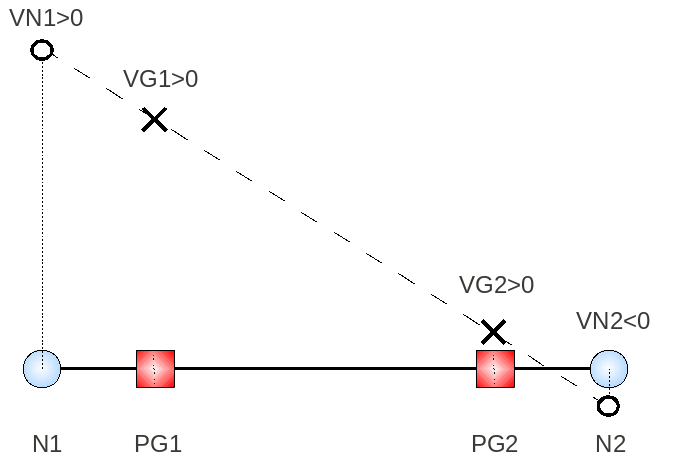
Figure 3: Extrapolation Disruption