3. Statistical post-processing#
3.1. Calculation of statistical quantities#
In the context of a Monte Carlo simulation approach, one is interested not only in a deterministic calculation result, but one wants to evaluate mean, median, standard deviation, fractile, and other statistics describing the output variable. In particular, this makes it possible to associate confidence intervals with the calculation results.
After having retrieved the sample of the outputs, we can use the preferred software (such as Open TURNS, the dedicated toolboxes of Python and Matlab, R) to perform these statistical post-treatments. Additionally, log-normal fragility curves can be evaluated using the Code_Aster operator POST_DYNA_ALEA. This is described in more detail in the next paragraph.
3.2. Calculation of fragility curves#
3.2.1. Definitions#
Fragility curves give the conditional probability of failure of a structure or component as a function of the seismic excitation level. The modeling and propagation of the uncertainties described above also allow the determination of fragility curves. All that is required is to introduce a failure criterion and to check at each Monte Carlo calculation whether the failure has been reached or not.
The main ingredients for the establishment of fragility curves by numerical simulation are the following:
Determination of the seismic excitation to be considered (accelerogram database),
Definition of failure criteria,
Uncertainty modeling and propagation by numerical simulation (Monte Carlo)
Estimation of the parameters (median and logarithmic standard deviation) of the log-normal fragility curve.
The fragility curve of a component can be defined from the concept of « capacity ». The capacity of a component is the value of the parameter representative of the seismic action from which the component is faulty. The current approach is to model capacity by a random variable according to a log-normal distribution, such as \(A\mathrm{=}{A}_{m}\varepsilon\), where \({A}_{m}\) is the median capacity and \(\varepsilon\) designates a log-normal random variable with a median unit and a logarithmic standard deviation \(\beta\). Also, the \(A\) capacity of a component (and \({A}_{m}\) thus its fragility curve), is characterized by two parameters which are the median (« median capacity ») and the standard deviation \(\beta\).
Thus, the probability of ruin for a given acceleration level \(a\) can be written as [bib3, bib2]:
Log-normal distribution \({P}_{f}(a)=\underset{0}{\overset{a}{\int }}\underset{}{\underset{\underbrace{}}{p(x)}}\text{dx}=\Phi (\frac{\text{ln}(a/{A}_{m})}{\beta })\)
where \(\Phi (\mathrm{.})\) refers to the distribution function of a reduced centered Gaussian random variable. The use of the lognormal model has the advantage of requiring a reduced number of simulations compared to a direct calculation of failure probabilities. Indeed, in a direct calculation, without a prior law hypothesis, it is necessary to determine the probabilities of rare events (the probabilities at the tail end of the distribution), which requires a very large number of Monte Carlo simulations. In what follows, we present two methods, maximum likelihood estimation and linear regression, to assess these two parameters.
If the damage or failure of a structure is characterized by a continuous variable of interest \(Y\), with a threshold \({Y}_{s}\), we can express the probability of failure (of the level of damage) for a level \(a\) earthquake as
\({P}_{f}(a)\mathrm{=}P(Y>{Y}_{s}\mathrm{\mid }a)\)
Classic damage variables \(Y\) for a concrete structure are drift (differential displacement between two floors of a building) or even the decrease in the first natural frequencies. The notations introduced here will be used for the evaluation of a fragility curve by linear regression (§3.2.2).
3.2.2. Maximum likelihood parameter evaluation#
In what follows, it is considered that the maximum acceleration was chosen to characterize the level of seismic excitation and therefore the capacity. The approach followed then consists in modeling the result of numerical experiments using a random Bernoulli variable \(X\). In fact, for each numerical simulation \(i\), we have two possible outcomes: either we have reached the critical level and we have failed (\({x}_{i}=1\)) or we have not failed (\({x}_{i}\mathrm{=}0\)). Likewise for each simulation, we can determine the value of the maximum acceleration \({a}_{i}\). The parameters of a fragility curve can be estimated using the maximum likelihood method. The likelihood function to be maximized for this problem is written as:
\(L\mathrm{=}\underset{i\mathrm{=}1}{\overset{N}{\Pi }}({P}_{f\mathrm{\mid }a}({a}_{i})){}^{{x}_{i}}{(1\mathrm{-}{P}_{f\mathrm{\mid }a}({a}_{i}))}^{1\mathrm{-}{x}_{i}}\)
In this expression, the \({x}_{i}\) achievement of \(X\) therefore takes the value 1 if there is a failure or 0 if there is no failure for the load (the maximum acceleration) \({a}_{i}\). These events happen with probability \({P}_{f\mid a}\) given by the expression (1). Parameter estimates \(\beta\) and \({A}_{m}\) are the ones that minimize \(-\text{ln}(L)\):
\(({\beta }_{C}^{e},{A}_{m}^{e})\mathrm{=}\text{arg}\underset{\beta ,{A}_{m}}{\text{min}}\left[\mathrm{-}\text{ln}(L)\right]\).
This step can be implemented by post-processing the calculation results. In the Code_Aster command file, you must, for each simulation, check whether there is a failure or not. For example, if the failure criterion consists of an allowable stress, it is checked whether the calculated maximum stress exceeds this stress.
Then, using CREA_TABLE, the results of the simulations are written in a results table. This table should contain two columns, PARA_NOCI and DEFA, which respectively fill in the value \({a}_{i}\) (the value PGA or any other indicator) and the value \({x}_{i}\) (\(1\) or \(0\)).
TAB1 = CREA_TABLE (LISTE =(
_F (PARA =” PARA_NOCI “, LISTE_R = PGA,),
_F (PARA =” DEFA “, LISTE_I =xi,),
),);
Note: If you enter a column DEMANDE instead of DEFA, then this column must contain the values of the seismic demand (variable of interest describing the failure or damage, for example a maximum stress or displacement).
TAB2 = CREA_TABLE (LISTE =(
_F (PARA =” PARA_NOCI “, LISTE_R = PGA,),
_F (PARA =” DEMANDE “, LISTE_I =request,),
),);
The keyword SEUIL must then be entered in POST_DYNA_ALEA to determine the continuation of the \({x}_{i}\).
The operator POST_DYNA_ALEA [U4.84.04] makes it possible to estimate the parameters of the lognormal fragility curve from the table TAB1via the keyword FRAGILITE:
TAB_POST = POST_DYNA_ALEA (FRAGILITE =( _F (TABL_RESU = TAB1,
AM_INI =0.3,
BETA_INI =0.1,
METHODE = “EMV”,
FRACTILE = (0.0,0.05,0.5,0.5,0.95,1.0),
NB_TIRAGE =Ns,
),),
TITRE = “curve 1”,
INFO =2,);
Initial values of the parameters \({A}_{m}\) and \(\beta\) to be estimated (starting point for the optimization algorithm) are given via AM_INI and BETA_INI. If the keyword FRACTILE is entered, the fractiles (confidence intervals) of the fragility curve are also determined by a resampling method (called the « bootstrap » method). Resampling consists of drawing new samples from the values of the original sample. These draws are at a discount, see [bib1] for more details. Next, the parameters of the fragility curve are determined for each « bootstrap » sample, which gives a sample of fragility curves. The fractiles for the sample of fragility curves obtained are then determined. In general, as many « bootstrap » samples are drawn as there are values in the original sample. However, it is possible to work with a lower number of draws by entering NB_TIRAGE (by default the number of draws corresponds to the size of the original sample, here \(\mathit{Ns}\)). In the example above, we therefore determine the envelope curves (fractions \(1.0\) and \(0.0\)) as well as the median \((0.5)\) and the fractiles at \(0.05\) and \(0.95\).
In the graph below, we give an example of a fragility curve for \({A}_{m}=0.68\) and \(\beta =0\text{.}\text{25}\):
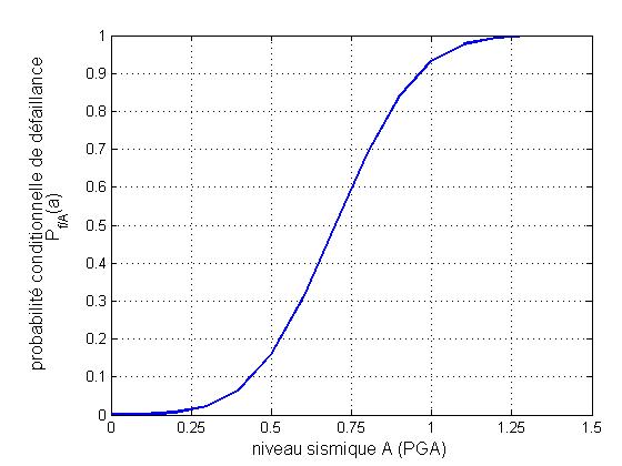
Figure 3.2.2-a: Conditional probability of failure as a function of PGA
3.2.3. Linear regression evaluation#
Regression is a very common method for determining the parameters of a log-normal fragility curve. It is mainly used in the United States to assess the fragility of civil structures such as roads, engineering structures and public buildings.
In this approach, we link the variable of interest \(Y\) (the drift for example), to the value of the seismic indicator \(a\) (for example the PGA) via a relationship of the type:
\(Y\mathrm{=}b{a}^{c}\eta\)
In the above expression, \(\eta\) is a log-normal random variable that can be defined using the reduced centered normal variable \(U\): \(\eta \mathrm{=}\mathrm{exp}(\beta U)\), and the variables \(b\) and \(c\) are the parameters of the model. These are obtained by a linear regression using the following expression:
\(\mathrm{ln}(Y)=\mathrm{ln}(b)+c\mathrm{ln}(a)+ϵ\)
where \(\epsilon\) is a normal random variable (Gaussian) centered with a standard deviation \(\sigma\) such as \(ϵ=\sigma U\). With these ratings, the probability of failure is written as a conditional probability, according to seismic level \(a\) and for a threshold \({Y}_{s}\):
\({P}_{f}(a)\mathrm{=}P(Y>{Y}_{s}\mathrm{\mid }a)\mathrm{=}1\mathrm{-}P(Y<{Y}_{s}\mathrm{\mid }a)\).
Taking into account the log-normal expression of the variable \(Y\), the analytic expression for the fragility curve is obtained:
\({P}_{f}(a)=\Phi \left(\frac{\text{ln}(b{a}^{c}/{Y}_{s})}{\sigma }\right)\)
Using the regression line, we can express the median threshold \({Y}_{s}\) from the median capacity as \({Y}_{s}\mathrm{=}b{a}_{s}^{c}\eta\). If we consider a critical « best-estimate » threshold that is assimilated to the median value in the uncertainty approach, we can note \({A}_{m}={a}_{s}\). The result is thus the expression of the log-normal fragility curve:
\({P}_{f}(a)=\Phi \left(\frac{\text{ln}(a/{A}_{m})}{\beta }\right)\)
where \(\beta =\sigma /c\) with the standard deviation of the regression error \(\sigma\). In practice, the value of the median capacity can be deduced directly from the regression curve and is expressed from the parameters of this last one as
\({A}_{m}\mathrm{=}\mathrm{exp}\left[\frac{\mathrm{ln}({Y}_{s}\mathrm{/}b)}{c}\right]\)
It is important to note that this model makes it possible to take into account heteroscedastic behavior (the variance of \(Y\) depends on the parameters of the model and is not constant).
The operator POST_DYNA_ALEA [U4.84.04] makes it possible to estimate the parameters of the lognormal fragility curve by regression from table TAB2 in §3.2.2 via the keyword FRAGILITE:
TAB_POST = POST_DYNA_ALEA (FRAGILITE =( _F (TABL_RESU = TAB2,
METHODE = “REGRESSION”,
SEUIL =0.05,
),),
TITRE = “curve 2”,
INFO =2,);
Experience shows that the dispersion (variability) of \(Y\) increases with the seismic level. On the other hand, unlike the maximum likelihood method, the logarithmic standard deviation does not depend on the threshold.
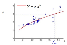
Figure 3.2.3-a: Example of a scatter plot and regression curve: Y variable as a function of PGA.