5. Links with parallelism#

Note: for more information you can consult the user manual dedicated to parallelism [U2.08.06].

5.1. Generalities#

Often a Code_Aster simulation can benefit from significant performance gains by distributing its calculations on several cores of a PC or on one or more nodes of a centralized machine.

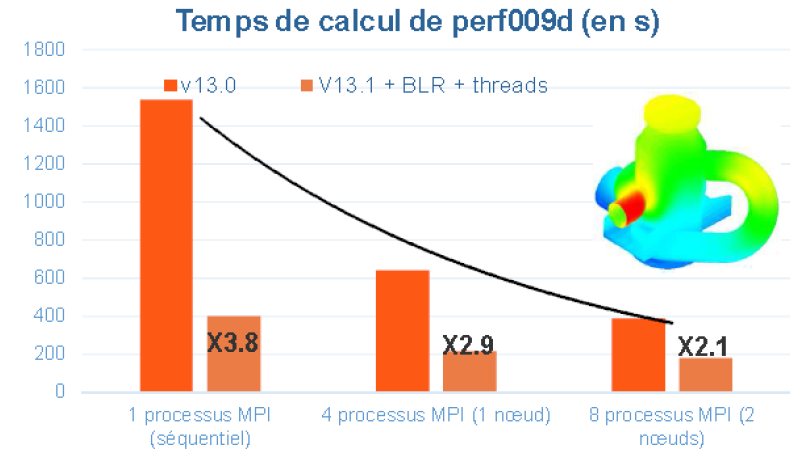
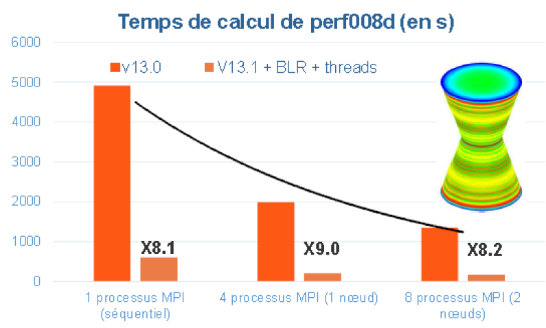
Figure 5.1.1._ Example of time savings provided by the parallelism MPI of Code_Aster v13.0, and with the hybrid one, MPI +OpenMP (+ low-rank compressions cf. [U4.50.01]) of Code_Aster v13.1. Comparisons made on the perf008d and perf009d performance test cases and on the Aster5 centralized machine.

You can save time (with parallelism MPI and with OpenMP parallelism) as well as in memory (only via MPI). These gains vary according to the functionalities requested, their settings, the data set and the software platform used: see figure 5.1.1.

In Code_Aster, by default, the calculation is sequential. But you can activate different parallelization strategies. These depend on the calculation step in question and on the settings chosen. They are often cumulative or chainable.

- We have three main classes of parallelizable problems, the second being the most common:

or the simulation can be organized into several**independent sub-calculations* (see §5.2),

or it’s not the case but:
this remains**dominated by linear or non-linear calculations* (operators STAT/DYNA/THER_NON_LINE, MECA_STATIQUE… cf. §5.3),

this remains**dominated by modal calculations* divisible into frequency sub-bands (INFO_MODE/CALC_MODES +” BANDE “, cf. §5.4).

To have an estimate of the time spent by an operator and therefore of the predominant steps of a calculation, you can activate the keyword MESURE_TEMPS of the DEBUT/POURSUITE commands (cf. [U1.03.03]) on a typical study (possibly shortened or diluted).

In all cases, it is advisable to divide the largest calculations into different steps in order to separate purely calculator ones [6] _ , those concerning displays, post-processing and field manipulations [7] _ .

5.2. Independent calculations#

When the simulation can be organized into different sub-calculations Aster independent (cf. figure 5.2.1) , the Astk [U1.04.00] tool offers an adapted functionality (cf. [U2.08.07]). It distributes these sub-calculations to various machine resources and retrieves their results. It is a completely « computer » parallel schema.

The limit being, for the moment, that all these unit calculations must each be able to be executed sequentially on the chosen machine (which can sometimes cause memory resource problems, cf. [U4.50.01]).

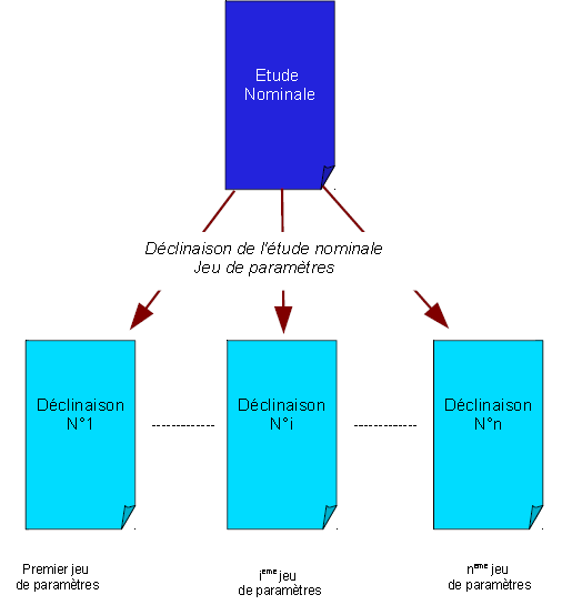
Figure 5.2.1._: Parallelism of independent calculations.

5.3. Parallelization of linear systems#

When this simulation cannot be broken down into similar and independent*Aster*sub-calculations, but it remains**dominated**nevertheless**by linear calculations**or**nonline* (operators STAT/DYNA/THER_NON_LINE,,,, MECA_STATIQUE,… cf. §5.3), we can organize a specific parallel schema.

It is based on the distribution of tasks and data structures involved in manipulating linear systems. Because it is these steps of building and solving linear systems that are often the most demanding in terms of calculation time and memory resources. They are present in most operators because they are buried in the depths of other « more professional » algorithms: non-linear solver, modal and vibratory calculation, time diagram…

The first step in the parallel diagram concerns the distribution of the model’s finite elements across all processes MPI. Each MPI process will therefore only manage the treatments and the data associated with the elements for which it is responsible. The construction of linear systems in Code_Aster (elementary calculations, assemblies) is then accelerated. We often talk about « parallelism in space ». It is a parallel diagram that is more of a « computer » nature.

Once these portions of the linear system have been constructed (cf. figure 5.3.1), two scenarios arise:

or the**following processing is naturally sequential* and therefore all MPI processes must have access to global information. To do this, these bits of linear systems are brought together and therefore the next step will not be accelerated, nor will its memory consumption decrease. It is most often an end of operator, post-processing, or a linear solver that is not parallelized in MPI (MULT_FRONT, LDLT, GCPC).

or the**following processing accepts parallelism MPI *, then it is mainly the linear solvers HPC MUMPS and PETSC. The parallel flow of data built up front is then transmitted to them (after some adaptations). These linear algebra packages then reorganize, internally, their own parallel schemes (with a more algebraic view). We then speak of a parallel diagram of a rather « numerical » order. This combination « computer parallelism », in terms of assembling the linear system, and, « numerical parallelism », in terms of its resolution, the 2*via* MPI, is the most common combination.

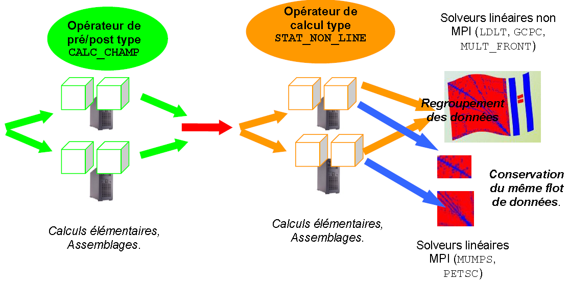
Figure 5.3.1._ Organization of the parallel diagram MPI for the construction and resolution of linear systems.

Notes:

Note that at the end of the cycle « construction of a linear system - resolution of this one », regardless of the scenario implemented (sequential or parallel linear solver MPI), the solution vector is then transmitted, in full, to all processes MPI. The cycle can thus continue regardless of the following configuration.

In addition, we can superimpose or substitute for this parallelism MPI (which works on all platforms), another level of parallelism managed this time by the OpenMP language. However, this is limited to machine fractions physically sharing the same memory (multi-core PCs or compute server nodes).

It does not make it possible to reduce memory consumption but on the other hand it accelerates certain types of calculation, with a lower granularity than that of MPI: it provides better acceleration even if the flow of data/processing is not very important. It is a parallel « computer » scheme that is mainly involved in the basic operations of linear algebra algorithms (via for example the BLAS library and some steps of the MUMPS solver).

This parallelism can be:

be combined with the MPI parallelism of MUMPS by speeding up the calculations within each MPI process. A hybrid parallel diagram with 2 levels is then obtained.
or replace parallelism MPI by speeding up the resolution of linear systems with MULT_FRONT.