7. Additional keyword information

The meaning of the various parameters of the SOLVEUR keyword are the subject of User documentation [:external:ref:`U4.50.01 <U4.50.01>`]. It must be synthetic to help the user in standard use of the code. For more advanced use, some additional information may be very useful. This chapter summarizes these items.

7.1. Singularity detection and keywords NPREC/STOP_SINGULIER/RESI_RELA

The essential step of direct solvers (SOLVEUR =_F (METHODE =” LDLT “/” MULT_FRONT “/” MUMPS “)) in terms of consumption. However, it can be difficult in two cases: the problem of constructing the factored matrix (structurally or numerically singular matrix) and numerical detection of a singularity (an approximated process that is more sensitive). The behavior of the code will depend on the case, the setting of NPREC/STOP_SINGULIER/RESI_RELA and the solver used. The combination of the cases is described in the attached table.

Type of solver/Type of problem	Construction of the factored
In case of a problem what happens? »	Digital detection of singularity (s) . In case of a singularity what happens?
LDLT/MULT_FRONT	Stop in ERREUR_FATALE	Case 1: We factor a dynamic matrix into a dynamics operator (see R5.01.01 §3.8, CALC_MODES… ): Stop in ERREUR_FATALE if it’s the algorithm’s work matrix. Issue of a ALARMEsi this is a stage of the Sturm test. In both cases STOP_SINGULIER has no impact on the process and NPRECdoit has no impact on the process and is positive. Case #2: If STOP_SINGULIER =” OUI “, Stop in ERREUR_FATALE in the post-processing phase of the linear solver. Case #3: If STOP_SINGULIER =” NON “, Issuance of a ALARME in the post-processing phase of the linear solver. Potentially inaccurate solution not detected by the linear solver. Apart from a possible encompassing process (Newton…) there are no digital safeguards to guarantee the quality of the solution. Case #4: If STOP_SINGULIER =” DECOUPE “, Start of the process of cutting the time step. You’re rebuilding a new problem for another time/load increment.
MUMPS	Stop ERREUR_FATALE	Case no. 1/4: If NPREC >0, same behavior as LDLT/MULT_FRONT (we find cases 1 to 4). <0 et RESI_RELA >**Case 5:** If #dnt_dgcebejjnifdkoppofklkgdiddogblok0, Singularity detection deactivated but the quality of the solution is measured in the linear solver. If the system is singular, its conditioning will be very high and the resolution quality will be very poor. If this resolution quality is higher than the value set in RESI_RELA: stop at ERREUR_FATALE. Case 6: If NPREC <0 and RESI_RELA <0, Singularity detection and solution quality measurement both disabled. Apart from a possible encompassing process (Newton…) we have no digital safeguards to guarantee the quality of the solution.

Table 7.1-1. Code behavior, depending on the configuration, when numerical factorization detects problems (poor data layout, numerical instabilities, strong conditioning, etc.) ) .

Some numerical details of the two types of singularity detection criteria (LDLT/MULT_FRONT versus MUMPS) are compared in the table below:

Features/Solver Type	LDLT / MULT_FRONT	MUMPS
Criterion	Local to each degree of freedom (relative value)	Global for all degrees of freedom
Test term	Absolute value of the diagonal term of each row	Infinite norm of the row/column of the row corresponding to the pivot
Detecting the line number (ISINGUdans the messages)	Always	Yes except when there are problems with the construction of the factored one
Providing the number of lost decimals	Yes, except when there are problems with the construction of the factored one	No
Deactivable	No	Yes

Table 7.1-2. Differences in singularity detection processes between solvers.

However, beyond differences in implementation and error messages (such solver points to one degree of freedom, another solver another degree of freedom), the two classes of direct solvers, LDLT/MULT_FRONT and MUMPS, generally conclude to the same type of diagnosis in case of problems [8] _ .

They point to a deficient data set: redundant or, on the contrary, absent blockages; overabundant linear relationships due to contact and friction; numerical data that is very heterogeneous (too large a penalty term) or illicit (negative Young’s modulus) or illicit numerical data (negative Young’s modulus… ) .

Notes:

• At worst, you must adjust the value of NPREC (increase or decrease by 1) to lead to the same observation. In general, the peculiarities are so obvious that the default setting is just fine.

• Unlike the other two solvers, * MUMPSne does not specify the number of decimal places lost, but activating its quality criterion (for example RESI_RELA =1.10-6) is an ultimate effective safeguard against this type of snag.

• It is normal and assumed that the degree of freedom detected is sometimes different when changing a numerical parameter (solver, renumber, preprocessing…) or computer parameter (parallelism…). It all depends on the order in which each processor treats the unknowns it is responsible for and what pivoting/balancing techniques may be implemented. In general, even different, the results contribute to the same diagnosis: to review the obstacles in its data creation.

• To get matrix conditioning [9] _

of its « raw » operator (that is to say without the possible pretreatments performed by the linear solver), we can use the combination MUMPS + PRETRAITEMENTS =” NON “+ INFO =2+ NPREC <0+ RESI_RELA >0. A very important value (> 10* 12) then betrays the presence of at least one singularity. On the other hand, while the additional cost of calculating the detection of a singularity is painless, that of estimating the packaging and the quality of the solution is less so (up to 40% in elapsed time; cf. §7.2.5) .

To be more precise, there are 9 distinct scenarios listed in the table below. They are based on exact or approximate nullity [10] _ « pivot » terms (cf. [R6.02.03] §2.3) selected by the numerical factorization phase of the direct solver in question. The first scenario appears during the numerical factorization itself (numerically or structurally singular matrix). The second case comes from the post-processing phase activated at the end of this numerical factorization.

As a matter of priority, the user should follow the advice provided by the alarm message (listed in the table below). If this is really not enough, the advanced user can try to play on the numerical parameters of the solver (renumber…), or even on the NPREC criterion when it comes to an almost zero pivot.

Table 7.1-3. Different cases of singularity detection and associated advice.

7.2. Solver MUMPS (METHODE =” MUMPS “)

7.2.1. Generalities

The solver MUMPS currently developed by CNRS/INPT - IRIT/-/INRIA/CERFACS is a direct multifrontend solver (in MPI) and robust, because it allows the rows and columns of the matrix to be rotated during numerical factorization.

MUMPS provides an estimate of the quality of the solution \(\text{u}\) (cf. keyword RESI_RELA) of the matrix problem \(\text{K}\text{u}=\text{f}\) via the notions of relative forward error (“relative forward error”) and inverse error (“backward error”). This “backward error”, \(\eta (\text{K},\text{f})\), measures the behavior of the resolution algorithm (when all is well, this real is close to machine precision, i.e. 10-15 in double precision). MUMPS also calculates an estimate of the conditioning of the matrix, \(\kappa (\text{K})\), which reflects the good behavior of the problem to be solved (real between 104 for a well-conditioned problem to 1020 for a very poorly conditioned problem). The product of the two is an increase in the relative error on the solution (“relative forward error”):

\(\frac{\parallel \delta u\parallel }{\parallel u\parallel }<{C}^{\mathrm{st}}\cdot \kappa (\text{K})\cdot \eta (\text{K},\text{f})\)

By specifying a strictly positive value to the RESI_RELA keyword (e.g. 10-6), the user indicates that he wants to test the validity of the solution of each linear system solved by MUMPS using this value. If the product \(\kappa (\text{K})\mathrm{\cdot }\eta (\text{K},\text{f})\) is greater than RESI_RELA the code stops at ERREUR_FATALE, specifying the nature of the problem and the offending values. With the INFO =2 display, we detail each of the terms of the product: \(\eta (\text{K},\text{f})\) and \(\kappa (\text{K})\).

To continue with the calculation, we can then:

• Increase the tolerance of RESI_RELA. For poorly conditioned problems, a tolerance of 10-3 is not uncommon. But it must be taken seriously because this type of pathology can seriously disturb a calculation (cf. next note on conditioning and §3.4).

• If it is the “backward error” that is too important: it is advisable to change the resolution algorithm. That is to say, in our case, to play on the parameters for launching MUMPS (TYPE_RESOL, PRETRAITEMENTS…).

• If operator conditioning is the culprit, it is advisable to balance the terms in the matrix, outside of MUMPS or*via* MUMPS (PRETRAITEMENTS =” OUI “), or to change the wording of the problem.

Note:

• Even in the very precise framework of solving linear systems, there are many ways to define the sensitivity to rounding errors of the problem in question (i.e. its conditioning). The one selected by MUMPS and, which is a reference in the field (cf. Arioli, Demmel and Duff 1989), is inseparable from the “backward error” of the problem. The definition of one does not make sense without defining the other. This type of conditioning should therefore not be confused with the concept of classical matrix conditioning.

On the other hand, the packaging provided by step MUMPS takes into account the SECOND MEMBRE of the system as well as the CARACTERE CREUX of the matrix. Indeed, it is not worth taking into account possible rounding errors on zero matrix terms and therefore not provided to the solver! The corresponding degrees of freedom do not « speak to each other » (seen from the finite element lens). Thus, this MUMPS conditioning respects the physics of the discretized problem. It does not plunge the problem back into the too rich space of full matrices.

Thus, the conditioning figure displayed by MUMPS is much less pessimistic than the standard calculation that another product can provide (Matlab, Python…). But let’s not forget that it is only his product with the “backward error”, called “forward error”, that is of interest. And only, as part of a linear system resolution via MUMPS.

7.2.2. Scope of use

It is a universal linear solver. It is deployed for all the functionalities of*Code_Aster.*

On the other hand, the use of solvers suffers from small limitations that are infrequent and that can be easily circumvented if necessary.

• In POURSUITEon mode only save code_aster FORTRAN objects to file and therefore not the occurrences of external products (MUMPS, PETSc). So be careful about the use of exploded commands in this context (NUME_DDL/FACTORISER/RESOUDRE). With MUMPS, it is not possible to FACTORISERou of the RESOUDREun linear system built during a previous Aster run (with NUME_DDL).

Likewise, we limit the number of simultaneous occurrences from MUMPS to NMXINS =50. When constructing his problem*via*exploded commands, the user must take care not to exceed this figure, otherwise the calculation stops in error. To do this, you can for example destroy the user concepts associated with matrices (for example*via the del command in .comm, cf. test case mumps03a.comm).

• With PETSc, on the other hand, this number is limited to 5, because the data structure is potentially richer and this library of iterative solvers is not commonly used in exploded commands (only in implicit operators that solve one or two linear systems simultaneously).

7.2.3. Parameter RENUM

This keyword allows you to control the tool used to renumber the linear system [11] _ . The Aster user can choose different tools divided into two families: the « frustrating » tools dedicated to one use and provided with MUMPS (“AMD”, “AMF”, “QAMD”, “PORD”), and, the « richer » and more « sophisticated » libraries that must be installed separately (“PARMETIS”/”METIS”, “PTSCOTCH”/”) SCOTCH “).

The choice of the renumber has a great importance on the memory and time consumption of the linear solver. If you want to optimize/adjust the numerical parameters linked to the linear solver, this parameter should be one of the first to try.

Product MUMPS breaks down its calculations into three steps (cf. [R6.02.03] §1.6): analysis, numerical factorization and down-ascent phase. In some cases, the analysis step may be predominant. Either because the problem is numerically difficult (numerous blockages, connections or contact areas, incompressible elements…), or because the other two steps have been very reduced thanks to parallelism (cf. [U2.08.06]). It may then be interesting to parallelize this analysis step (via MPI). This makes it possible to speed it up and reduce its memory consumption. This is done by choosing one of the proposed parallel renumbers: “PARMETIS” or “PTSCOTCH”.

The choice of such a parallel renumber, while it often improves the performances of the analysis step of MUMPS, may nevertheless degrade those of the following two other steps MUMPS. However, if the main problem was to reduce the memory consumption of this analysis step or if the following steps of MUMPS benefit from sufficient parallelism (or compression, cf. parameters ACCELERATION/LOW_RANK_SEUIL), the balance can be generally positive.

On the other hand, during parallel modal calculations (operator CALC_MODES), we sometimes observed disappointing speed-ups due to an inappropriate choice of renumber. In this case it was found that the choice of a « sophisticated » renumber was counterproductive. It is better to impose a simple “AMF” or “QAMD” on MUMPS, rather than “METIS” or “PARMETIS” (often taken automatically in “AUTO” mode).

7.2.4. Parameter ELIM_LAGR2

Historically, Code_Aster’s direct linear solvers (“MULT_FRONT” and “LDLT”) did not have a pivoting algorithm (which seeks to avoid the accumulation of rounding errors by division by very small terms). To get around this problem, the way in which boundary conditions are taken into account by Lagranges (AFFE_CHAR_MECA/THER…) has been modified by introducing double Lagranges. Formally, we are not working with the initial matrix \({\mathrm{K}}_{0}\)

\({\mathrm{K}}_{0}\mathrm{=}\left[\begin{array}{cc}\mathrm{K}& \mathrm{blocage}\\ \mathrm{blocage}& 0\end{array}\right]\begin{array}{c}\mathrm{u}\\ \mathrm{lagr}\end{array}\)

but with its doubly dualized form \({\mathrm{K}}_{2}\)

\({K}_{2}=\left[\begin{array}{ccc}K& \mathrm{blocage}& \mathrm{blocage}\\ \mathrm{blocage}& -1& 1\\ \mathrm{blocage}& 1& -1\end{array}\right]\begin{array}{}u\\ {\mathrm{lagr}}_{1}\\ {\mathrm{lagr}}_{2}\end{array}\)

Hence an additional memory and calculation cost.

As MUMPS has pivoting capabilities, this choice to dualize boundary conditions can be called into question. By initializing this keyword to “OUI”, we only take into account one Lagrange, the other being a spectator [12] _ . Hence a \({\mathrm{K}}_{1}\) work matrix that is simply dualized.

\({K}_{1}=\left[\begin{array}{ccc}K& \mathrm{blocage}& 0\\ \mathrm{blocage}& 0& 0\\ 0& 0& -1\end{array}\right]\begin{array}{}u\\ {\mathrm{lagr}}_{1}\\ {\mathrm{lagr}}_{2}\end{array}\)

smaller because the extra-diagonal terms of the rows and columns associated with these spectator Lagranges are then initialized to zero. *Conversely, with the value “NON”, MUMPS receives the usual dualized matrices.

For problems with many Lagranges (up to 20% of the total number of unknowns), activating this parameter is often expensive (smaller matrix). But when this number explodes (> 20%), this process can be counterproductive. The gains made on the matrix are cancelled out by the size of the factorized one and especially by the number of late pivots that MUMPS must perform. Imposing ELIM_LAGR2 =” NON “can then be very interesting (for example: gain of 40% in CPU on the mac3c01 test case).

We unplugg also temporarily unplug this parameter when we want to calculate the determinant of the matrix, because otherwise its value is distorted by these changes in the blocking terms. The user is notified of this automatic configuration change by a dedicated message (visible in INFO =2 only).

7.2.5. Parameter RESI_RELA

Default value=-1.d0 in non-linear and in modal,1.d-6 in linear.

This setting is disabled by a negative value.

By specifying a strictly positive value for this keyword (for example 10-6), the user indicates that he wants to test the validity of the solution of each linear system solved by MUMPS using this value.

This careful approach is recommended when the solution is not itself corrected by another algorithmic process (Newton algorithm, singularity detection…) in short in the linear operators THER_LINEAIRE and MECA_STATIQUE. In non-linear terms, the singularity detection criterion and the Newton correction are sufficient safeguards. We can therefore unplug this control process (this is what is done by default via the value -1). In modal, this detection of singularity is an algorithmic tool for capturing natural modes. This detection is the subject of a dedicated configuration specific to each method.

If the relative error on the solution estimated by MUMPS is greater than resi the code stops at ERREUR_FATALE, specifying the nature of the problem and the offending values.

Activating this keyword also initiates an iterative refinement process whose objective is to improve the solution obtained. This post-processing has a specific configuration (keyword POSTTRAITEMENTS). It is the solution resulting from this iterative improvement process that is being tested by RESI_RELA.

Note:

• This control process involves the estimation of the matrix conditioning and some feedback from the iterative refinement post-processing. It can therefore be quite expensive, especially in OOC, due to I/O RAM /disk during downhill runs (up to 40%). When enough safeguards are implemented, it can be unplugged by initializing resi to a negative value.

7.2.6. Settings to optimize memory management (MUMPS and/or JEVEUX)

In general, a large part of the calculation times and memory peaks RAM of a Code_Aster simulation are attributable to linear solvers. The linear solver MUMPS is no exception to the rule but the richness of its internal configuration and its fine coupling with Code_Aster provide the user with a certain flexibility. In particular with regard to the management of memory consumption RAM.

In fact, during a memory peak occurring for a linear system resolution via MUMPS, memory RAM can be broken down into 5 parts:

• JEVEUX objects except the matrix,

• The JEVEUX objects associated with the matrix (generally SD MATR_ASSE and NUME_DDL),

• MUMPS objects used to store the matrix,

• MUMPS objects allowing you to store the factored one,

• Auxiliary MUMPS objects (pointers, vectors, communication buffers…).

Roughly speaking, part 4 is the most cumbersome. In particular, it is much bigger than the parts 2 and 3 (factor of at least 30 due to the filling phenomenon cf. [R6.02.03]). The latter are equivalent in size but one is exercised in the space allocated to JEVEUX, while the other lives in the complementary space allocated by the task manager to the job. As for the other two parts, 1 and 5, they often play a marginal role [13] _ .

To reduce these memory consumption, the Aster user Aster has several lever arms (most of the time cumulative):

• Centralized parallel computing on n cores (part 4 divided by \(n\)) or distributed (parts 3 and 4 divided by \(n\)).

• Distributed parallel computing + MATR_DISTRIBUEE ** (limited scope of use): parts 3 and 4 divided by \(n\), part 2 divided by slightly less than \(n\).

The activation of the* OOC of**** MUMPS ** (keyword GESTION_MEMOIRE =” OUT -OF- CORE “): part 4 decreases by 2/3.

Knowing that before each call to the “analysis+numerical factorization” cycle of MUMPS, we systematically unload the largest JEVEUX objects from part 2 onto disk.

Tips:

In view of the above elements, an obvious tactic is to switch the calculation to distributed parallel mode (value by default) rather than sequential. The centralized parallel mode does not contribute anything from this point of view [14] _ , it is not a step to consider. If, however, we remain dependent on a particular mode, here are the tips associated with each:

• In sequential mode: the main gains will come from activating GESTION_MEMOIRE =” OUT_OF_CORE “(on reasonably sized problems).

• In distributed parallel mode: after about ten processors, the OUT_OF_CORE no longer provides much gain. MATR_DISTRIBUEE can then help in some situations.

If these strategies do not provide sufficient gains, we can also try non-linearly (at the cost of possible losses in precision and/or time) to relax the resolution of the linear system (FILTRAGE_MATRICE, MIXER_PRECISION) or even those of the encompassing process (elastic tangent matrix, reduction of the modal projection space…). If the matrix is well conditioned and if you do not need to detect the singularities of the problem (so no modal calculation, buckling…), you can also try an iterative solver (GCPC/PETSC + LDLT_SP).

Table 7.2-1. Synopsis of the various solutions permitting

to optimize memory during a calculation with MUMPS .

Keyword GESTION_MEMOIRE =” OUT_OF_CORE “

To activate or deactivate the OOC capabilities of MUMPS which will then entirely unload on disk the real part of the factorized blocks managed by each processor. This functionality can of course be combined with parallelism, resulting in a greater variety of operations to adapt to execution contingencies. OOC, like parallelism, helps to reduce RAM memory requirements per processor. But of course (a bit) at the expense of time CPU: price to pay for I/O for one, for MPI communications for the other.

Attention: During a parallel calculation, if the number of processors is large, the size of objects MUMPS that can be unloaded on disk becomes small. The transition to OOC can then be counterproductive (low gain in RAM and additional time cost) compared to the IC mode set by default.

This phenomenon occurs all the sooner the smaller the size of the problem is small and it is all the more sensitive the more we do a lot of descents and ascents [15] _ in the solver.

Broadly [16] _ , below 50.103 degrees of freedom per processor and if you have enough RAM (3 or 4 GB) per processor, you can probably switch to IC.

Notes:

• For now, during an execution MUMPS in OOC, only the real vectors containing the factored one are (entirely) unloaded onto disk. The integer vectors accompanying this data structure (of just as large size) do not yet benefit from this mechanism. On the other hand, this unloading only takes place after the analysis phase of MUMPS. In short, in very big cases (several million degrees of freedom), even with this OOC, memory contingencies can prevent calculation. In principle, we leave with a ERREUR_FATALE documented.

• In MUMPS, in order to optimize memory occupancy, most integers are coded in INTEGER 4*. Only integers corresponding to a memory address are transcribed in*INTEGER*8*. This makes it possible to address larger problems, on 64-bit architectures. this cohabitation of short/long integers to optimize memory space has been extended to certain large objects JEVEUX .

• When Code_Aster has finished assembling the working matrix, before passing « the relay » to MUMPS, it unloads to disk the largest objects JEVEUX related to the resolution of the linear system ( SMDI /HC, /HC, DEEQ, HC,, NUEAQ, VALM.*..). This is in order to leave as much RAM space as possible for MUMPS. In mode*GESTION_MEMOIRE =” AUTO “, if this memory space is not sufficient for MUMPS to work in IC, this partial release of objects*JEVEUX*is completed by a general release of all the releasable objects (i.e. not open for read/write). This operation can provide a lot of gains when you « drag » a lot of peripheral objects*JEVEUX*into memory (field projection, long transient…). On the other hand, this massive unloading can waste time. In particular in parallel mode due to bottlenecks in the access cores/ RAM. *

Keyword MATR_DISTRIBUEE

This parameter can be used in operators MECA_STATIQUE, STAT_NON_LINE,, DYNA_NON_LINE,, THER_LINEAIRE, and THER_NON_LINE with AFFE_CHAR_MECA or AFFE_CHAR_CINE . It is only active in distributed parallel ( AFFE_MODELE/DISTRIBUTION/METHODE equals other than CENTRALISE ). This feature can of course be combined with GESTION_MEMOIRE =” OUT_OF_CORE “, resulting in a greater variety of operations to adapt to execution contingencies.

In parallel mode, when distributing data JEVEUX upstream of MUMPS, you do not necessarily recut the data structures concerned. With the option MATR_DISTRIBUEE =” NON “, all distributed objects are allocated and initialized at the same size (the same value as sequentially). On the other hand, each processor will only modify the parts of objects JEVEUX for which it is responsible. This scenario is particularly suited to the distributed parallel mode of MUMPS (mode by default) because this product groups these incomplete data streams internally. Parallelism then makes it possible, in addition to saving in calculation time, to reduce the memory space required by resolution MUMPS but not that required to build the problem in JEVEUX.

This is not a problem as long as RAM space for JEVEUX is much less than that required by MUMPS. Since JEVEUX mainly stores the matrix and MUMPS stores its factored (usually dozens of times bigger), the calculation bottleneck RAM is theoretically on MUMPS. But as soon as you use a few dozen processors in MPI and/or activate OOC, as MUMPS distributes this factorized by processor and unloads these pieces onto disk, the « ball comes back into the court of JEVEUX ».

Hence option MATR_DISTRIBUEE, which resizes the matrix, more precisely non-zero terms for which the processor is responsible. The JEVEUX space required then decreases with the number of processors and falls below the RAM required at MUMPS. The results in Figure 7.2-1 illustrate this gain in parallel on two studies: a RIS Pump and the Epicure tank.

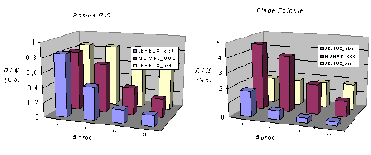
Figure 7.2-1: Evolution of consumption RAM (in GB) according to the number of processors, Code_Aster v11.0 ( JEVEUX standard MATR_DISTRIBUE =” NON “and distributed, resp.” OUI “) and MUMPS OOC. Calculations carried out on a Pump RIS (perf009) and on the Epicure study tank (perf011) .

Notes:

• Here we treat data resulting from an elementary calculation (RESU_ELEM and CHAM_ELEM) or from a matrix assembly (MATR_ASSE). The assembled vectors (CHAM_NO) are not distributed because the memory gains induced would be low and, on the other hand, as they are involved in the evaluation of numerous algorithmic criteria, this would involve too many additional communications.

• In mode MATR_DISTRIBUE, to make the join between the end of MATR_ASSE * local to the processor and the global MATR_ASSE (which we do not build), we add an indirection vector in the form of a NUME_DDLlocal.

7.2.7. Parameters to reduce calculation time via various acceleration/compression techniques

Keywords ACCELERATION and LOW_RANK_SEUIL

These two keywords activate and pilot MUMPS acceleration/compression techniques. These can significantly reduce the computation time of large studies, without restricting the scope of use, and with potentially little or no impact on the accuracy, robustness and overall behavior of the simulation.

They are generally only useful for large problems (N at least > 2.106ddls). The gains observed on some performance test cases and Aster studies vary from 20% to 80% (examples in figures 7.2-2/7.2-3). They increase with the size of the problem, its massive nature and they are complementary to those provided by parallelism and the renumber.

The description of these functionalities in the document [U4.50.01] is completed here.

When you have chosen an acceleration based on “low-rank” compressions (“LR” and “LR+” values of the keyword ACCELERATION), you must define the rate of these compressions. This rate is indicated by the keyword LOW_RANK_SEUIL. It controls the truncation criterion of the numerical compression algorithm [17] _ . Broadly, the larger this number, for example 10-12 or 10-9, the greater the compression will be and therefore the more interesting the time savings can be.

However, if this value is too big (for example >10-9), the factored matrix may be approximated too much and the solution vector may thus prove to be too inaccurate! In a non-linear process it’s not always that bad because the encompassing Newton algorithm can correct the situation!

On the other hand, in linear mode or to deal with numerically difficult problems (incompressible finite elements, X- FEM…), it is then necessary to ensure that the resolution includes the corrective post-processing procedure (cf. iterative refinement, keyword POSTTRAITEMENTS). <0) est souvent à privilégier par rapport au choix par défaut (POSTTRAITEMENTS =” AUTO “+ RESI_RELA >In this case, in this case where when trying to establish a compromise between performance and precision, the value POSTTRAITEMENTS =” MINI “(+ RESI_RELA0).

To be exhaustive, note that the real value of this keyword can also be zero, the compression will then be done with machine precision, or become negative, the compression will then use the relative threshold.

\(∥\mathrm{K}∥\times \mid \text{lr\_seuil}\mid\)

The first value allows you to benefit from a little compression without any impact on precision (for functional tests or expertise).

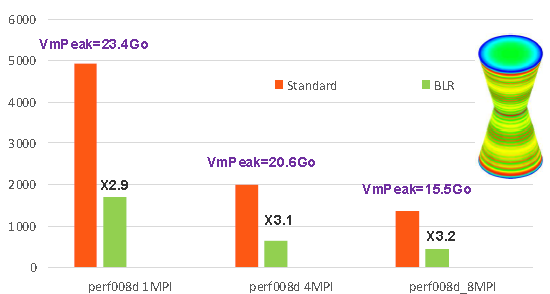
Figure 7.2-2: Example of gains provided by low-rank compressions on the perf008d performance test case (parameters by default, memory management in OOC, N=2M, NNZ =80M, =80M, Facto_ METIS4 =80M, Facto_ =7495M, conditioning=10 7*). As a function of the number of MPI processes activated, we plot the elapsed times consumed by the entire linear system resolution step in Code_Aster v13.1, its memory peak RAM, as well as the acceleration factor provided by BLR.*

In summary, the criterion for approximating the compression algorithms of MUMPS is set according to the following rule:

If LOW_RANK_SEUIL =0.D0:

truncation to machine precision.

If LOW_RANK_SEUIL >0.D0:

the truncation of compression algorithms uses lr_threshold directly.

If LOW_RANK_SEUIL <0.D0:

the truncation of the compression algorithms is based on the relative threshold mentioned above.

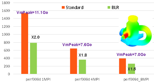
Figure 7.2-3: Example of gains provided by low-rank compressions on the perf009d performance test case (parameters by default, memory management in OOC, N=5.4M, NNZ =209M, =209M, Facto_ METIS4 =209M, Facto_ =5247M, conditioning=10 8*). As a function of the number of MPI processes activated, we plot the elapsed times consumed by the entire linear system resolution step in Code_Aster v13.1, its memory peak RAM, as well as the acceleration factor provided by BLR.*

Notes:

• For now, the gains from low-rank compressions only concern the second calculation step of MUMPS, that of numerical factorization, which is often the most expensive. These gains therefore depend on the importance of this step compared to the other steps of the linear solver (construction NUME_DDL, analysis and descend-ascent). Recall that we can easily trace the cost of this factorization step (item #1 .3) by activating the detailed monitoring of the time costs of each calculation step (keyword DEBUT/MESURE_TEMPS/ [U1.03.03]).

• Apart from the compression tools themselves, the low-rank strategy involves two additional costs, one in the analysis step [18] _

and the other at the end of numerical factorization [19] _ . But when it comes to major problems, they are generally quickly offset by the gains made by this technique.

• For the moment, these gains only concern calculation time, memory consumption remains similar or even slightly higher (auxiliary vectors for compression) than those of a standard “full-rank” calculation.

• For reasonable compression thresholds (<10-9) the impact on the quality of the results and on the related “outputs” (detection of singularity, calculation of determinants and the Sturm criterion…) are often negligible [20] _

. Beyond that, it is no longer completely guaranteed. The good behavior and robustness of the calculation may suffer. This setting should be limited to a « relaxed » direct solver or preconditioner use [21] _ for an iterative Krylov solver.

[1]

Cf. Test case error03a and error04a.

[2]

In the sense of solving a sparse linear system, cf. papers by M.Arioli/J.Demmel/I.Duff.

[3]

Controlled by NPREC (cf. [U4.50.01] §3.2).

[4]

In order, in particular, to limit the phenomenon of filling the factorized one, cf. [R6.02.03] §1.7.

[5]

To maintain the consistency of data structures and maintain a certain computer readability/maintainability, it is better to « bluff » the usual process by moving from \({\mathrm{K}}_{2}\) to \({\mathrm{K}}_{1}\), rather than to the optimal scenario \({\mathrm{K}}_{0}\).

[6]

But not always. So part 1 can end up being expensive when calculating a lot of time steps, when loading projected fields or when a behavioral law manipulates a lot of internal variables. Likewise, part 5 may become non-negligible during a parallel calculation on a large number of processors.

[7]

It is mainly used to test and validate new developments as well as parallel studies.

[8]

For example, in a STAT_NON_LINE with lots of Newton iterations and/or iterative refinement iterations.

[9]

A lot depends on the study.

[10]

Variant with truncation of a QR factorization: RRQR for “Rank Revealing QR”.

[11]

Pre-selection of eligible dense blocks and construction of related data structures.

[12]

The compressed dense blocks are decompressed after use before starting the final descent-ascent stage, because this is still processed in “full-rank”. In the long term, it will also be treated in “low-rank” and this additional cost will disappear.

[13]

Concerning, the quality of the result is all the more true if the post-processing procedure has been activated.

[14]

Future functionalities: for example for use as a « relaxed » direct solver (cf. keywords FILTRAGE_MATRICE/MIXER_PRECISION) or as a preconditioner (cf. methods PETSc/GCPC + LDLT_SP).