5. Examples of use

5.1. Introduction

Next, we present five examples on mesh adaptation. These examples have different educational goals. The first example, which is the most recent, comes from a study carried out at EDF R&D on an HP rotor. The following three examples remain more academic but aim to show a particular aspect of the adaptation process. Finally, the last example illustrates the cutting mode chosen by HOMARD (this is a particular situation encountered by a user who was surprised by the final mesh).

Educational objective of each example

Rotor HP: showing the need to take border monitoring into account when adapting

Elastic flexure beam:

Know how to interpret the results of the MACR_INFO_MAIL command in the .mess file

Illustrate the value of free refinement compared to uniform refinement

Use mechanical error indicators and choose the right component (absolute or relative)

Thermal cylinder head:

Use thermal error indicators and observe refined areas according to the component of the selected indicator

Very simplified representation of the dudgeonned tube plate (thermoplastic calculation):

Show the value of a free adaptation compared to a uniform adaptation on calculation times

In thermal, give the python command file allowing to do mesh adaptation in transient

Locating band in a plate: understanding the cutting mode chosen by HOMARD

Note:

When doing mesh adaptation, it is useful to have some knowledge of the Python language in order to avoid the repetition of commands. In the test case ZZZZ121a .comm, we will find an example of a Python loop.

5.2. HP rotor study

Background:

This study was carried out at department AMA in 2006 as part of the Nuclear Fleet Steam Turbine Lifespan Project. Very briefly, the aim is to locate the areas of maximum stress encountered on the HP rotor (FIG. 5.2-a) of a turbine and to numerically assess the stress level in order to verify whether there is a risk of a crack starting from corrosion under stress. In order to rule on the risk of cracking by CSC, several models were carried out, including one in 2D axisymmetric of the complete rotor with an aspect on the quality of the mesh. We refer the reader to document [bib12] for more information on this study; our objective here is to highlight only the mesh aspect.

Study approach:

This study focuses on the maximum constraints obtained numerically in order to compare them with threshold constraints resulting from experimental tests. Von Mises stress analysis is first of all required because this type of stress is always greater than the relevant components of the stress tensor. Thus, when the Von Mises stresses are less than the threshold stresses, it is considered that the risk of CSC cracking is unlikely in the absence of impurities. However, when the Von Mises stresses are greater than the cracking threshold by CSC, it becomes necessary to analyze the maximum values of the stress tensor more finely, as well as the main stresses in order to assess the margins in relation to the risk of cracking by CSC.

Modeling:

The behavior of the material is elastic. The load is of the centrifugal force type due to rotation. The calculation is done with the command STAT_NON_LINE. The initial mesh is free and very fine in the areas of curvature, in order to obtain the most reliable stress values possible. The elements are quadrilaterals of degree two. The mesh includes 71037 elements and 217198 nodes.

Result:

Here we look at the areas where the Von Mises stress is maximum. The most stressed zone is located near the coupling on the bearing side AVANT, in the zone of curvature of the groove between the coupling and the rest of the rotor (zone A). The other areas loaded with stress are located at the level of the connection of the attachments to the rotor (zone B and C, for example).

Wings

Figure 5.2-a: partial view of the rotor and blades

Mesh adaptation:

In order to validate the level of stresses obtained in the most loaded zone (zone A) and in two of the rotor/fin connection zones (zones B and C), a mesh adaptation is carried out with the absolute term of the residual error indicator and a criterion in percentage of finite element.

Two results are presented below:

• one without border tracking: division of 5% of elements with the greatest error,

• and the other with border tracking: division of 2% of elements. The border mesh makes it possible, through its great discretization, to define very precisely the curved areas of the geometry.

The table shows all the observed changes in the Von Mises constraint in areas A, B and C during the adaptation process without border monitoring.

Mesh number	1 (initial)	2	3	4
Number of meshes	71037	94469	126622	171905
Number of nodes	217198	283192	361692	480643
Stress in zone A	0.946	1	1	1	1
Stress in zone B	0.566	0.662	0.699	0.723
Stress in zone C	0.446	10.554	0.626	0.681

Table 1: evolution of Von Mises constraints without border monitoring

The table below shows the same results but with border tracking.

Mesh number	1 (initial)	2	3	4	5
Number of meshes	71037	79857	79857	88085	98332	109678
Number of knots	217198	237108	237108	259755	288871	320348
Stress in zone A	0.946	0.946	0.946	0.946	0.946	0.946
Stress in zone B	0.566	0.675	0.675	0.662	0.662
Stress in zone C	0.446	0.446	0.584	0.584	0.644	0.644

Table 2: Evolution of Von Mises constraints with border monitoring

Without border monitoring, we note that:

• in zone A, the stress stabilizes from the second mesh;

• on the other hand, in zones B and C, the stress does not stabilize. This phenomenon is associated with a lack of discretization of this curved zone which creates a geometric discontinuity. Without border tracking, remeshing does not make it possible to correct this problem and even accentuates the geometric discontinuity, which has the effect of increasing the stress.

With border monitoring, we notice that:

• The constraint in zone A does not change. This consistency is due to the reduction in the number of cells taken into account during the refinement. In fact, since the results obtained around zone A do not form part of the 2% of cells presenting the largest error, no refinement is made in this zone and the constraint then remains constant. The value to be taken into account for the maximum stress is therefore that presented in table 6.1-a.

• Border monitoring helps to stabilize the Von Mises constraints in areas B and C.

Conclusion:

This analysis shows two important lessons. First, it is risky to rely uncritically on the results of a calculation carried out on a single mesh. We can see here that with the initial mesh, although quite fine to the eye, the values obtained are far from being final. By modifying the mesh, they evolve until they stabilize. You should not deprive yourself of these additional calculations, especially since they are simple to set up and perform automatically. Then, we note the advantage of monitoring borders if the geometry has curved areas.

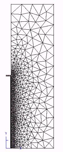
5.3. Elastic flexure beam

This example has been used during training courses. It is a test case of the Code_Aster database that can be found under the FORMA tests.

Modeling:

It is a metal beam (steel 16 MND5, \(E={210.10}^{3}\mathrm{Mpa}\), \(\nu =0.2\)) in bending. The calculation is elastic (MECA_STATIQUE or STAT_NON_LINE) in plane stress modeling (C_ PLAN). The initial mesh is either in TRIA3 or in TRIA6.

Figure 5.3-a: Bending beam calculation diagram

Using MACR_INFO_MAIL :

Using this command provides the following information (.mess):

ANALYSE FROM MAILLAGE

=====

Mesh to be analyzed

MA_0

Creation date: Friday, September 27, 2002 at 3:58pm 20 pm

Size: 2

Degree: 1

It's a starting point.


Direction | Unit | Minimum | Maximum

--------------------------------------------------

X | UNKNOWN | 0. | 100.00

Y | UNKNOWN | 0. | 10,000

INTERPENETRATION DES ELEMENTS

=====


**********************************************************

**

*Summary of the active faces*

**

*No problems have been encountered.*

**

**********************************************************


QUALITE DES ELEMENTS

===== =====

**********************************************************

*Quality of the triangles in the calculation mesh*

*Reminder: the quality is equal to the diameter ratio*

*of the triangle on the radius of the inscribed circle,*

*normalizes to 1 for a regular triangle.*

**********************************************************

*Minimum: 1.0117 Maximum: 2.0158*

**********************************************************


**********************************************************

*Distribution function*

**

*Values* Number of elements*

*Mini < < Maxi* per class *cumulative*

* *in%. number* in%. number *

**********************************************************

*1.00 < 1.05* 14.75. 9 *14.75. 9*

*1.05 < 1.10* 42.62. 26 *57.38. 35*

*1.10 < 1.15* 16.39. 10 *73.77. 45*

*1.15 < 1.20* 1.64. 1 *75.41. 46*

*1.20 < 1.25* 6.56. 4 *81.97. 50*

*1.25 < 1.30* 11.48. 7 *93.44. 57*

*1.30 < 1.35* 0.00. 0.0 *93.44. 57*

*1.35 < 1.40* 3.28. 2 *96.72. 59*

*1.40 < 1.45* 0.00. 0 *96.72. 59*

*1.45 < 1.50* 0.00. 0 *96.72. 59*

*1.50 < 1.55* 0.00. 0 *96.72. 59*

*1.55 < 1.60* 0.00. 0 *96.72. 59*

*1.60 < 1.65* 0.00. 0 *96.72. 59*

*1.65 < 1.70* 0.00. 0 *96.72. 59*

*1.70 < 1.75* 1.64. 1 *98.36. 60*

*1.75 < 1.80* 0.00. 0 *98.36. 60*

*1.80 < 1.85* 0.00. 0 *98.36. 60*

*1.85 < 1.90* 0.00. 0 *98.36. 60*

*1.90 < 1.95* 0.00. 00 *98.36. 60*

*1.95 < 2.00* 0.00. 0 *98.36. 60*

*2.00 < 2.05* 1.64. 1 *100.00. 61*

*2.05 < 2.10* 0.00. 0 *100.00. 61*

*2.10 < 2.15* 0.00. 0 *100.00. 61*

*2.15 < 2.20* 0.00. 0 *100.00. 61*

*2.20 < 2.25* 0.00. 0 *100.00. 61*

*2.25 < 2.30* 0.00. 0 *100.00. 61*

*2.30 < 2.35* 0.00. 0 *100.00. 61*

*2.35 < 2.40* 0.00. 0 *100.00. 61*

*2.40 < 2.45* 0.00. 0 *100.00. 61*

*2.45 < 2.50* 0.00. 0 *100.00. 61*

*2.50 < inf.* 0.00. 0 *100.00. 61*

**********************************************************


NOMBRE OF ENTITES OF CALCUL

===== === =====


**********************************************************

*The knots*

**********************************************************

*Total number* 48*

**********************************************************


**********************************************************

*The stitches-point*

**********************************************************

*Total number* 2*

**********************************************************


**********************************************************

*The areas*

**********************************************************

*Total number* 15*

*. including insulated edges* 0*

*. including edge edges of 2D regions* 15 *

*. including edges internal to faces/volumes* 0*

**********************************************************


**********************************************************

*The faces*

**********************************************************

*Total number* 61*

**********************************************************


CONNEXITE DES ENTITES FROM CALCUL

==== ==== ====


**********************************************************

*The faces are in a single block.*

**********************************************************


TAILLES DES SOUS - DOMAINES OF CALCUL

===== =====


Management | Unit

-------------------------

X | UNKNOWN

Y | UNKNOWN


**********************************************************

*2D subdomains*

**********************************************************

*Number* Name*Surface*

**********************************************************

*-4* FAMILLE_MAILLE_ -4_______________ *1000.0*

**********************************************************

*Total:* 1000.0*

**********************************************************


**********************************************************

*1D subdomains*

**********************************************************

*Number* Name*Length*

**********************************************************

*-3* FAMILLE_MAILLE_ -3_______________ *10,000*

*-2* FAMILLE_MAILLE_ -2_______________ *50,000*

*-1* FAMILLE_MAILLE_ -1_______________ *40.000*

**********************************************************

*Total:* 100.00*

**********************************************************

We learn from this message:

• the extreme coordinates of the mesh;

• the absence of interpenetration problems;

• a histogram of the geometric quality of the cells (we will observe the good quality of this mesh);

• the number of knots, stitches, points, edges, faces;

• the connectivity of the mesh;

• the size of the domains defined by the groups of cells (this description is not very readable, however, it will be observed that the 2D domain of the beam has an area of 1000 as expected).

Using MACR_ADAP_MAIL option UNIFORME:

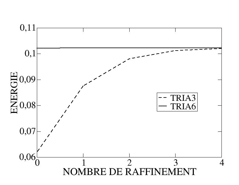
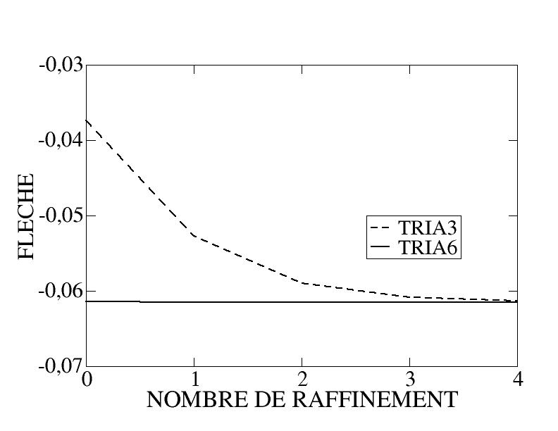
Let us observe the results obtained, by comparing a linear mesh (TRIA3) and a quadratic mesh (TRIA6), the initial mesh being shown in the figure. On the curves showing the evolution of the energy and the deflection of the beam as a function of the refinement number (Figure), two conclusions can be drawn:

• on the one hand, the quadratic elements demonstrate their obvious superiority;

• on the other hand, remeshing (here very simplistic since it is uniform) proves its interest: the initial linear mesh being very far from being sufficiently refined, remeshing makes it possible to obtain good results after a few iterations.

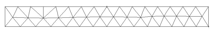
Figure 5.3-b: Initial mesh

Figure 5.3-c: Evolution of arrow and energy with the number of refinements

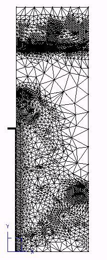
Using MACR_ADAP_MAIL option RAFFINEMENT:

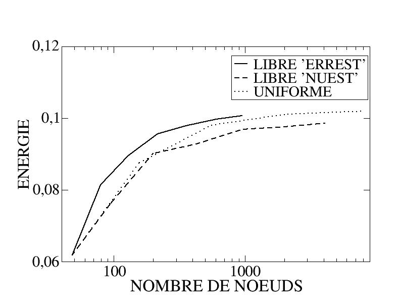
The first question to address when using free refinement with HOMARD is the choice of the field that will be used as a criterion for dividing the elements. In this example, an error indicator is used. Following the principles set out in the advice paragraph, the choice was made to use the residual indicator (even if in this case, we are within the scope of use of the Zhu-Zienkiewicz indicators). In contrast, this example compares the absolute and standardized components of the indicator to illustrate the caution required in using the standardized component.

The mesh is linear here in order to clearly illustrate the effect of mesh adaptation, because we saw previously that the initial mesh already gives good quality results with elements of order 2.

If we compare the energy results with the « absolute » component (“ERREST”) and the « relative » component (“”) and the « relative » component (“NUEST”) as a function of the number of nodes (figure where we added the same evolution for uniform refinement), we observe: - free refinement with the absolute component converges more quickly to the reference than uniform refinement (hence the interest in doing free refinement); - free refinement with the relative component converges more slowly to the reference than the uniform refinement, which at first glance is surprising.

Figure 5.3-d: Evolution of energy as a function of the number of nodes

This last point can be explained by drawing the three fields from the error indicator, which is done in the figures, and. It is clear that the fact that the norm of the standardized stress is low in an area (neutral fiber of the beam in particular) where refinement is less necessary than elsewhere (see the absolute error) makes the result of normalization \({e}_{{E}_{\text{REL}}}=\text{100}\times \frac{{e}_{E}}{\sqrt{{e}_{E}^{2}+{\parallel {\sigma }_{h}\parallel }_{E}^{2}}}\) random. Indeed, it should be noted that areas with zero normalization constraints will be considered to have an error of 100%: if it is necessary to refine in this zone, it will be good (although it will mask the other areas to be refined), if the refinement is less necessary, it will be bad. It is therefore necessary to analyze your problem carefully before using the relative component of the error indicator, since the absolute component can be considered to be more reliable. In particular, it seems to us that the use of the normalized error is only possible after analysis by the user of the normalization constraint map.

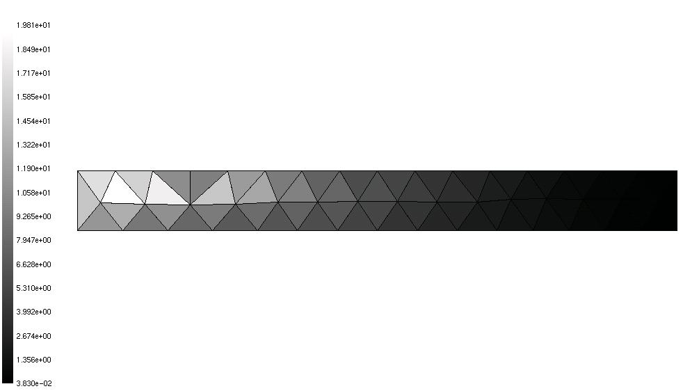
Figure 5.3-e: Absolute component

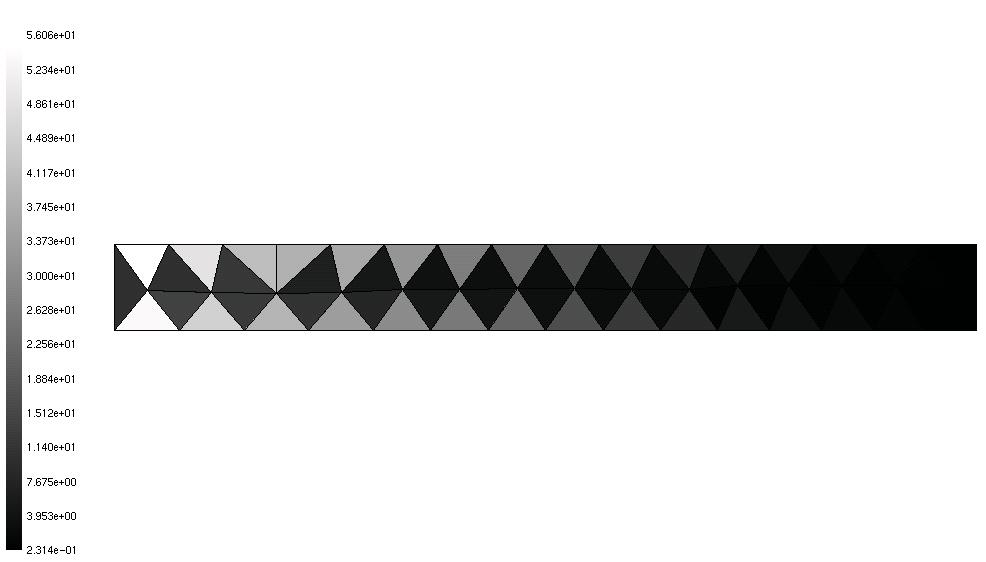
Figure 5.3-f: Normalization constraint standard

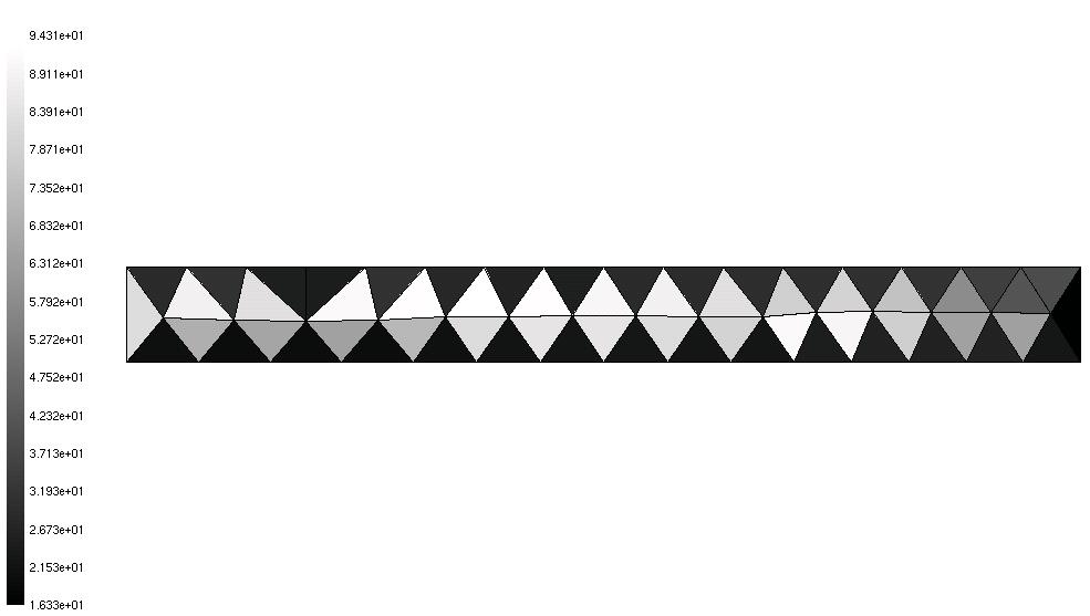
Figure 5.3-g: Standard component

5.4. Thermal cylinder head

The following structure is considered:

Figure 5.4-a: Diagram of the cylinder head calculation

subject to the following loads:

Figure 5.4-b: Diagram of cylinder head calculation loads

We are only interested here in the thermal part to highlight the possibility of using the decomposition of the various error terms. Indeed, in the context of « standard » use (i.e. when all the error terms are of interest to the user), it will be necessary to choose the total error (“ERTABS” or “ERTREL”); on the other hand, if the user is particularly interested in taking into account the boundary conditions well into account, he can thus guide the refinement by using the various terms, flow or exchange in this case.

The initial mesh (figure) verifies one of our tips: start from a « reasonable » mesh.

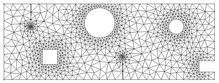
Figure 5.4-c: Initial mesh

If we refine the total relative error (“ERTREL”), figure:

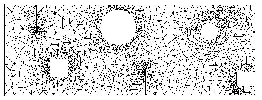
Figure 5.4-d: Refined mesh based on total relative error

and a refinement on the term relative exchange (“TERME2”), figure:

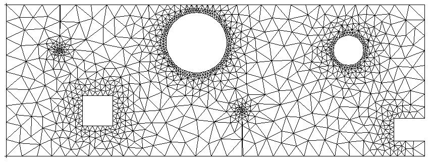
Figure 5.4-e: Refined mesh based on the relative error on the trade term

It is obvious that the adapted meshes differ greatly. In the second case, refinement has indeed been oriented towards the holes, which are the seat of exchange conditions.

5.5. Thermoplastic example

We consider the following structure of revolution (modelled axisymmetrically):

Figure 5.5-a: Thermoelastic calculation diagram

where the parts that are gray are plastic, the rest are elastic. Charging is applied in 2 steps:

• the first consists of a purely mechanical loading (pressure on the zone with arrows on the diagram), with a charging phase followed by a discharge phase;

• the second consists of a temporary thermal loading (exchange condition on the lower and upper parts of the structure).

Remeshing strategy and moment list:

The loading is discretized according to a list of moments, so the question arises: what strategy should be adopted with respect to remeshing? In fact, depending on the case treated, we can:

• remount at each calculation step: the mesh is then adapted to each calculation step individually. It is then necessary to project the fields of one mesh onto the other;

• remount only once, at the end of the calculation, and start the calculation again from the beginning with the new mesh.

The first strategy is to be adopted in the case where the refinement zones change a lot, as we will see an example in the following thermal calculation; the second can be adopted in the case where the refinement zones change little, as in this mechanical case where it is a question of following the growth of a plastic zone.

Mechanical calculation:

For mechanical calculation, the following strategy is therefore adopted:

• calculation of the entire list of moments;

• remeshing;

• repeat (1 & 2) until satisfactory result.

It is not so much the implementation in Code_Aster that is interesting in this case (which differs from previous implementations only in that there are several moments of calculation) as the results obtained by adapting the mesh to a non-linear case.

To judge the contribution of the remeshing, let’s look at the radial stresses on the segment separating the two regions (figure) which are compared to a « reference » obtained by 3 uniform remeldings: the gain of remeldings based on the error indicator is visible.

Figure 5.5-b: Post-treatment location

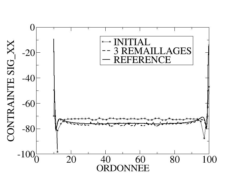
Figure 5.5-c: Stress Profile

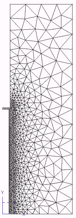
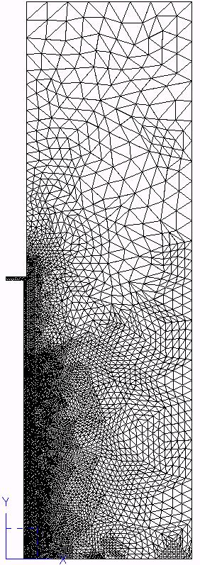
The figure shows the initial mesh and the mesh after 3 re-meshes based on the error indicator.

An indication of the variations in the size (and therefore the time) of the resolutions between the reference calculation (3 uniform refinements) and the calculation with 3 refinements based on the error indicator is given in table 3.

	Number of nodes	Calculation time
Reference mesh	175,000	~3000 s
3 free refinements (i.e. 4 calculations)	8,500	~60 s

Table 3: Performance Indication

Figure 5.5-d: Initial mesh and after 3 adaptations

Thermal transient calculation:

In this case, it is a question of calculating a thermal transition, two exchange conditions being imposed at the bottom and at the top of the structure. As the zone that will present a strong temperature gradient will move within the structure (advanced by one front), the strategy adopted for re-meshing will take this into account: the mesh must be updated regularly during the transition. In practice, the list of moments is subdivided into blocks, within these blocks of calculation moments the mesh will be the same (and the remeshing occurs at the end of the block). So there are 3 nested loops:

• the loop over the N blocks of moments;

• the loop on the reinforcements of the current block;

• the loop (hidden in THER_LINEAIRE) on the moments of the block.

If we look at the results at the last calculated moment, in particular the temperature on the post-treatment line already used in mechanics (figure), we note the advantage of mesh adaptation. As can be seen on the initial meshes and adapted to the last time step, figure, the mesh has not changed in the vicinity of the sampling line: the improvement in the calculated temperature comes from the zones that have been refined elsewhere.

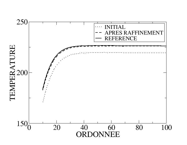
Figure 5.5-e: Initial mesh Temperature Profile

Figure 5.5-f: Initial mesh Initial mesh and the last calculation time step

5.6. Plate with a location band

Modeling:

It is a rectangular plate that is subjected to compression. The behavior of the material is softening (negative isotropic work hardening, law “DRUCKER - PRAGER”). The calculation is done with the command STAT_NON_LINE. The mesh consists of QUAD8. Because of the softening behavior, a band of localization of the cumulative plastic deformation is observed. Inside this band, the behavior is plastic and the plasticity indicator is 1, outside this band, the behavior remains elastic and the plasticity indicator is equal to 0.

Adaptation process:

The adaptation of the mesh is carried out with the plasticity indicator (third internal variable V3 of the law of DRUCK_PRAGER). The division criterion chosen is a threshold value set at 0.5 (keyword “CRIT_RAF_ABS”). This ensures refinement in the location area, the user’s objective in this study.

MACR_ADAP_MAIL (

ADAPTATION = 'RAFFINEMENT',

MAILLAGE_N = MAIL_INI,

MAILLAGE_NP1 = co ('MAIL_FIN'),

RESULTAT_N = water,

NOM_CHAM = “VARI_ELGA”, NOM_CMP = “V3”,

CRIT_RAFF_ABS = 0.5,)

Redistricting result:

All the stitches are cut in four, even in the elastic zone. This result, which may seem surprising at first glance, is due to the division method adopted by HOMARD and in particular to the compliance rules (see § 2.3). Figures and figures illustrate this result.

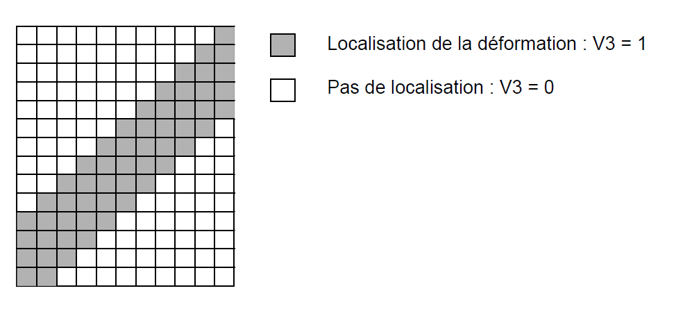
Figure 5.6-a: Initial mesh

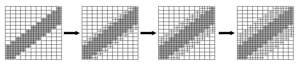
Figure 5.6-b: Breakdown of the gray zone and then compliance gradually