5. Some calculation examples#
Three cases are presented to illustrate the implementation of the technique.
The first case corresponds to a standard modal calculation using operators CREA_ELEM_SSD and ASSE_ELEM_SSD.
The second case corresponds to a transient response calculation. A double projection is performed. The first projection is executed when the dynamic macro element is created and the second projection is performed on the generalized model of the structure assembled for the response calculation.
The third case corresponds to a harmonic response calculation on a dissipative structure. The sequence of elementary operators necessary for the creation of dynamic macroelements and the assembly of generalized substructure matrices is described.
5.1. An example of modal calculation#
This is modeling and test case SDLS106 [V2.03.106].
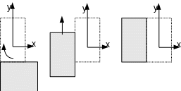
In this test case, we want to calculate the natural modes of a structure composed of two substructures defined in two different frames of reference. The association of these two substructures is supposed to obtain a plate in a condition supported on its edges.
It can be schematized as follows:
Substructure 1 |
Substructure 2 |

|

|
The assembled structure is a rectangular plate resting on these edges.

To achieve this assembled structure, the substructure 2 is rotated and translated. In fact, the two substructures must be expressed in the same frame of reference.

Rotation -90 degrees around DZ + Translation following DY
The steps for creating the dynamic macroelement of substructure 1 will be presented. The dynamic macroelement of substructure 2 is created in an analogous manner.
Definition of boundary conditions for substructure 1:
We want to use a Craig-Bampton type base, so we must embed the degrees of freedom of the interface that are associated here with the group of nodes GAUCHE. The other conditions correspond to the boundary conditions of the substructure.
CHARGE_1 = AFFE_CHAR_MECA (MODELE = MODELE1, DDL_IMPO =(
_F (GROUP_NO = “BLOQUE”, DX = 0.0, DY = 0.0, DZ = 0.0),
_F (GROUP_NO = “GAUCHE”, DX = 0.0, DY = 0.0, DZ = 0.0,
DRX = 0.0, DRY = 0.0, DRZ = 0.0),
_F (GROUP_NO = “BAS”, DX = 0.0, DY = 0.0, DZ = 0.0),
_F (GROUP_NO = “HAUT”, DX = 0.0, DY = 0.0, DZ = 0.0)))
Creation of the dynamic macro element:
The CREA_ELEM_SSD operator is used to create the dynamic macroelement,
We have a distributed interface here, we want to use interface modes as link modes. Under the keyword factor BASE_MODALE, we choose a RITZ base and enter the number of interface modes to use.
The keyword factor CALC_FREQ provides information on the number of normal modes to use.
MACEL1 = CREA_ELEM_SSD (
MODELE = MODELE1,
CHARGE = CHARGE_1,
CHAM_MATER = CHAMAT1,
CARA_ELEM = PARAM1,
INTERFACE = _F (NOM = “GAUCHE”,
TYPE = “CRAIGB”,
GROUP_NO = “GAUCHE”),
BASE_MODALE = _F (TYPE = “RITZ “,
NMAX_MODE_INTF = 20,),
CALC_FREQ = _F (NMAX_FREQ = 6,),
)
In the same way, the dynamic macro-element of the substructure 2 is created.
Assembly of the various substructures:
The substructures are assembled using the operator ASSE_ELEM_SSD
The keyword factor RESU_ASSE_SSD makes it possible to assign a name to the result concepts (model, generalized ddl numbering, generalized matrices).
The keyword factor SOUS - STRUCT allows you to name the various substructures. It is in this factor keyword that we affect the possible rotation and translation of the macro-element (we first perform the rotation ANGL_NAUT and then the translation TRANS).
The LIAISON keyword defines the interfaces between substructures. In the case where interface modes are used as connection modes, REDUIT must be specified under the OPTION keyword.
The group of elements GROUP_MA_MAIT_ * controls the displacement field at the interface. If the interfaces are not compatible (the knots are not facing each other), it is advisable to choose the finest mesh as the master stitch. Otherwise, by default, the cells in substructure 1 are defined as master cells.
Choice ELIMINE under the METHODE keyword means that we number the generalized degrees of freedom by taking into account the bond equations by the method of eliminating constraints.
ASSE_ELEM_SSD (
RESU_ASSE_SSD = _F (
MODELE = CO (“MODEGE”),
NUME_DDL_GENE = CO (“NUMEGE”),
RIGI_GENE = CO (“RIGGEN”),
MASS_GENE = CO (“MASGEN”),
),
SOUS_STRUC = (
_F (NOM = “CARRE1”,
MACR_ELEM_DYNA = MACEL1,),
_F (NOM = “CARRE2”,
MACR_ELEM_DYNA = MACEL2,
ANGL_NAUT = (-90.,0.,0.),),
TRANS = (0.,0.5,0. ),
),
LIAISON = (
_F (SOUS_STRUC_1 = “CARRE1”,
INTERFACE_1 = “GAUCHE”,
GROUP_MA_MAIT_1 = “CALCUL”,
OPTION = “REDUIT”,
SOUS_STRUC_2 = “CARRE2”,
INTERFACE_2 = “BLOQUE”,),
),
VERIF = _F (STOP_ERREUR = “OUI”,
PRECISION = 1.E-6,
CRITERE = “RELATIF”),
METHODE = “ELIMINE”,
),
Calculation of the natural modes of the assembled structure:
The modal calculation is carried out on the assembled generalized matrices. The modal deformations obtained are expressed in generalized coordinates.
RESGEN = CALC_MODES (MATR_RIGI = RIGGEN,
MATR_MASS = MASGEN,
OPTION = “PLUS_PETITE”,
CALC_FREQ =_F (NMAX_FREQ =10,),
SOLVEUR_MODAL =_F (METHODE =” SORENSEN “,),
VERI_MODE =_F (PREC_SHIFT =5.0E-3,
STOP_ERREUR =” NON “,
STURM =” NON “,
SEUIL =9.9999999999999995E-01),
STOP_BANDE_VIDE =” NON “,
)
Restitution on a physical basis:
To exploit the results, it is necessary to return them on a physical basis.
MODCOT1 = REST_SOUS_STRUC (RESU_GENE = RESGEN,
TOUT_ORDRE =” OUI “,
SOUS_STRUC =” CARRE1 “,);
MODCOT2 = REST_SOUS_STRUC (RESU_GENE = RESGEN,
TOUT_ORDRE =” OUI “,
SOUS_STRUC =” CARRE2 “,);
Quality control of results:
The quality of the results obtained can be checked by verifying the continuity of movements at the interface. This makes it possible to validate the number of interface modes chosen.
In this test case, the displacement of the node N9 of the substructure 1 is compared to that of the node N70 of the substructure 2. These two nodes are facing each other.
T1_DZ= POST_RELEVE_T (ACTION =_F (INTITULE =” CARRE1 “,
NOEUD =( “N9”),
RESULTAT = MODCOT1,
NOM_CHAM =” DEPL “,
TOUT_ORDRE =” OUI “,
NOM_CMP =”DZ”,
OPERATION =” EXTRACTION “,
),);
T2_DZ= POST_RELEVE_T (ACTION =_F (INTITULE =” CARRE2 “,
NOEUD =( “N70”),
RESULTAT = MODCOT2,
NOM_CHAM =” DEPL “,
TOUT_ORDRE =” OUI “,
NOM_CMP =”DZ”,
OPERATION =” EXTRACTION “,
),);
F_DZ= FORMULE (NOM_PARA =( “DZ_C1”, “DZ_C2”,),
VALE =”abs (DZ_C1 - DZ_C2) “)
TC_DZ = CALC_TABLE (TABLE =T1_DZ,
ACTION =( _F (OPERATION =” RENOMME “,
NOM_PARA =( “DZ”, “DZ_C1”),),
_F (OPERATION =” COMB “,
TABLE =T2_DZ,
NOM_PARA =( “NUME_ORDRE”,),),
_F (OPERATION =” RENOMME “,
NOM_PARA =( “DZ”, “DZ_C2”),),
_F (OPERATION =” OPER “,
NOM_PARA =” ECART “,
FORMULE =F_DZ),
),
TITRE =”Comparing DZ ssd 1/ssd 2”)
TEST_TABLE (
TABLE = TC_DZ,
NOM_PARA = “ECART”,
TYPE_TEST = “SOMM”,
VALE = 0. ,
CRITERE = “ABSOLU”,
PRECISION = 3.E-3,
REFERENCE = “ANALYTIQUE”,)
Here we calculate the sum of the absolute values of the differences. The keyword PRECISION defines the maximum allowed deviation.
It is also possible to check the invalidity of the work of the liaison forces using the CALC_CORR_SSD operator. This calculation consumes quite a lot of CPU time.
CALC_ENR = CALC_CORR_SSD (MODELE_GENE = MODEGE,
RESU_GENE = RESGEN,
SHIFT =1. ,
UNITE =6)
A summary of the results obtained is stored, by default, in the message file. We can enrich the database if we see that the work of the liaison forces is not negligible. We can draw inspiration from modeling a of test case SDLS122 [V2.03.122] for the implementation of this enrichment of the projection base.
5.2. An example of calculating a transient response#
This is modeling and test case SDLD102 [V2.01.102].
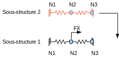
Substructures are composed of discrete elements. The first substructure is stressed by a point force.
The same model and the same mesh are used to define the two substructures.

The complete structure is obtained by assembling the two substructures.

Definition of the boundary conditions of the substructure:
We want to use a classic Craig-Bampton basis, the node at the interface must be blocked (node \(\mathit{N3}\) for substructure 1 and node \(\mathit{N1}\) for substructure 2).
CHARGE_L = AFFE_CHAR_MECA (MODELE = MODELE,
DDL_IMPO =(
_F (NOEUD =”N2”,
DY=0. ,
DZ=0. ,
DRX =0. ,
DRY =0. ,
DRZ =0.,),
_F (NOEUD =”N1”,
DX=0.,),
_F (NOEUD =”N3”,
DX=0.,),),);
Creation of dynamic macroelements:
The load \(\text{FX}\) is applied to this substructure 1, it is then necessary to enter a numbering for the degrees of freedom of the substructure. This numbering will be used later when defining the load on the assembled model.
MACEL1 = CREA_ELEM_SSD (
MODELE = MODELE,
CARA_ELEM = PARAM,
CHARGE = CHARGE_L,
CHAM_MATER = CHAMAT,
NUME_DDL =CO (“NUMDDL_L”),
INTERFACE =_F (NOM =” DROITE “,
TYPE =” CRAIGB “,
NOEUD =”N3”,),
BASE_MODALE = _F (TYPE = “CLASSIQUE “,),
CALC_FREQ = _F (NMAX_FREQ = 1,),
)
Creation of the dynamic macro element of substructure 2:
MACEL2 = CREA_ELEM_SSD (
MODELE = MODELE,
CARA_ELEM = PARAM,
CHARGE = CHARGE_L,
CHAM_MATER = CHAMAT,
INTERFACE =_F (NOM =” GAUCHE “,
TYPE =” CRAIGB “,
NOEUD =”N1”,),
BASE_MODALE = _F (TYPE = “CLASSIQUE “,),
CALC_FREQ = _F (NMAX_FREQ = 1,),
)
Assembly of the various substructures:
ASSE_ELEM_SSD (
RESU_ASSE_SSD = _F (
MODELE = CO (“MODEGE”),
NUME_DDL_GENE = CO (“NUMEGE”),
RIGI_GENE = CO (“RIGGEN”),
MASS_GENE = CO (“MASGEN”),
),
SOUS_STRUC =( _F (NOM =” COTE1 “,
MACR_ELEM_DYNA = MACEL1,),
_F (NOM =” COTE2 “,
MACR_ELEM_DYNA = MACEL2,
TRANS =( 0.2,0.,0.),),),
LIAISON =_F (SOUS_STRUC_1 =” COTE1 “,
INTERFACE_1 =” DROITE “,
SOUS_STRUC_2 =” COTE2 “,
INTERFACE_2 =” GAUCHE “,),
VERIF =_F (STOP_ERREUR =” OUI “,
PRECISION =1.E-6,
CRITERE =” RELATIF “,),
);
Calculation of the transient response of the assembled structure:
Definition and assembly of the load vector:
CHARTRAN = AFFE_CHAR_MECA (MODELE = MODELE,
FORCE_NODALE =_F (NOEUD =”N2”,
FX=1.,),);
V_ ELEM = CALC_VECT_ELEM (OPTION =” CHAR_MECA “,
CHARGE = CHARTRAN,);
The load must be expressed in the same numbering as the projection vectors (numbering the degrees of freedom of substructure 1).
V_ ASSE = ASSE_VECTEUR (VECT_ELEM =V_ ELEM,
NUME_DDL = NUMDDL_L,);
Assembling the load vector on the generalized model (loading applied to the substructure COTE1):
FGEN = ASSE_VECT_GENE (NUME_DDL_GENE = NUMEGE,
CHAR_SOUS_STRUC =_F (SOUS_STRUC =” COTE1 “,
VECT_ASSE =V_ ASSE,),);
Definition of the projection base for the transient response calculation (in the majority of cases, the base is composed of the system’s natural modes):
RESGEN = CALC_MODES (MATR_RIGI = RIGGEN,
MATR_MASS = MASGEN,
OPTION =” PLUS_PETITE “,
CALC_FREQ =_F (NMAX_FREQ =3,),
TITRE =” CALCUL DES MODES PROPRES FROM THE STRUCTURE GLOBALE “,
);
Numbering the degrees of freedom of the calculation base:
NUMEMODE = NUME_DDL_GENE (BASE = RESGEN,
STOCKAGE =” DIAG “,);
Projection of the matrices assembled on the basis of calculation:
MASPRO = PROJ_MATR_BASE (BASE = RESGEN,
NUME_DDL_GENE = NUMEMODE,
MATR_ASSE_GENE = MASGEN,);
RIGPRO = PROJ_MATR_BASE (BASE = RESGEN,
NUME_DDL_GENE = NUMEMODE,
MATR_ASSE_GENE = RIGGEN,);
Load projection based on calculation:
VECPRO = PROJ_VECT_BASE (BASE = RESGEN,
NUME_DDL_GENE = NUMEMODE,
VECT_ASSE_GENE = FGEN,);
By default, the movement and the speed are zero at the initial moment. How to capture the initial condition of the system is shown below.
The field is created on the mesh of the substructure with the same numbering as that of the macro-element.
CHAMP_0 = CREA_CHAMP (OPERATION =” AFFE “, TYPE_CHAM =” NOEU_DEPL_R”,
MAILLAGE = MAILLA,
NUME_DDL = NUMDDL_L,
AFFE =_F (TOUT = “OUI”,
NOM_CMP = (“DX”, “DY”, “DZ”, “DZ”, “DRX”, “DRY”, “DRZ”,),
VALE = (0.,0.,0.,0.,0.,0.,0.,))
)
Projection of the field onto the assembled generalized model:
VGEN_0 = ASSE_VECT_GENE (NUME_DDL_GENE = NUMEGE,
CHAR_SOUS_STRUC =_F (SOUS_STRUC =” COTE1 “,
VECT_ASSE = CHAMP_0,),);
Second projection of the field based on response calculation:
DEPINI = PROJ_VECT_BASE (BASE = RESGEN, VECT_ASSE_GENE = VGEN_0,
NUME_DDL_GENE = NUMEMODE,
TYPE_VECT =” DEPL “)
VITINI = PROJ_VECT_BASE (BASE = RESGEN, VECT_ASSE_GENE = VGEN_0,
NUME_DDL_GENE = NUMEMODE,
TYPE_VECT =” VITE “)
The transient response calculation can be done using the DYNA_VIBRA command. The projection resolution technique is used on a computational basis.
Calculation of the transient response on the projected assembled model:
TRANGEN1 = DYNA_VIBRA (TYPE_CALCUL =” TRAN “, BASE_CALCUL =” GENE “,
SCHEMA_TEMPS =_F (SCHEMA =” EULER “,),
MATR_MASS = MASPRO,
MATR_RIGI = RIGPRO,
INCREMENT =_F (INST_INIT =0. ,
INST_FIN =82. ,
PAS =0.01,),
ETAT_INIT =_F (DEPL = DEPINI,
VITE = VITINI,),
ARCHIVAGE =_F (PAS_ARCH =10,),
EXCIT =_F (VECT_ASSE = VECPRO,
COEF_MULT =1.,),);
Restitution on a physical basis:
The results can be reproduced directly on the substructure or on a visualization mesh called a skeleton mesh that must be defined beforehand.
Creation of the visualization mesh:
SQUEL = DEFI_SQUELETTE (MODELE_GENE = MODEGE,
SOUS_STRUC =( _F (NOM =” COTE1 “,
GROUP_MA =” RESSORT “
),
_F (NOM =” COTE2 “,
GROUP_MA =” RESSORT “
),),);
Restitution of the calculation base on the visualization mesh:
MODGLO = REST_SOUS_STRUC (RESU_GENE = RESGEN,
TOUT_ORDRE =” OUI “,
SQUELETTE = SQUEL,);
Restitution of the response on the visualization mesh (for a resolution with double projection, do not forget to specify the reproduction of the calculation base on the substructure or on the skeleton):
TRAN1 = REST_GENE_PHYS (RESU_GENE = TRANGEN1,
MODE_MECA = MODGLO,
LIST_INST = LIST_R,
INTERPOL =” LIN “,
TOUT_CHAM =” OUI “,
NOEUD =” NO3 “,);
We therefore recall that for a temporal response calculation, a double projection is performed. A first projection of the substructure based on normal modes and link modes and a second projection of the reduced assembled model based on response calculation.
5.3. An example of harmonic response calculation#
In the majority of cases, a harmonic response calculation is performed on a dissipative model. Operators CREA_ELEM_SSD and ASSE_ELEM_SSD only deal with conservative structures. In this example, we detail the underlying elementary operations, necessary for carrying out a harmonic response calculation by dynamic substructuring.
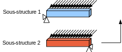
Test case SHLV301A is used to illustrate the presentation. It is a rectangular bar modelled with quadratic solid elements. Sinusoidal pressure is applied to a lateral face of the bar.

The assembled structure:

Definition and assignment of the material:
MAT = DEFI_MATERIAU (ELAS =_F (RHO = 7.8E03, NU = 0.3, E = 2.1E11,
AMOR_ALPHA = 1.6E-5, AMOR_BETA = 16.))
CHMAT = AFFE_MATERIAU (MAILLAGE = MAYA,
AFFE =_F (TOUT = “OUI”,
MATER = MAT))
Loading description:
PRESSION = AFFE_CHAR_MECA (
MODELE = POVOL,
PRES_REP =_F (GROUP_MA = “PRESSION”,
PRES = 50.E4))
Description of the boundary conditions (We want to use a Mac Neal projection base: the nodes of the interface are free):
FIXAT1 = AFFE_CHAR_MECA (
MODELE = POVOL,
DDL_IMPO =(
_F (GROUP_NO = “COND1”, DY = 0. ),
_F (GROUP_NO = “CONDZG”, DZ = 0. ),
_F (NOEUD = “N26”, DX = 0. ),
_F (GROUP_NO = “DROITE”, X = 0.)))
Creation of dynamic macroelements:
Creation of the elementary matrices of substructure 1:
K_ ELEM1 = CALC_MATR_ELEM (MODELE = POVOL,
CHAM_MATER = CHMAT,
OPTION =” RIGI_MECA “,
CHARGE =( FIXAT1,)
)
M_ ELEM1 = CALC_MATR_ELEM (MODELE = POVOL,
CHAM_MATER = CHMAT,
OPTION =” MASS_MECA “,
CHARGE =( FIXAT1,)
)
A_ ELEM1 = CALC_MATR_ELEM (MODELE = POVOL,
CHAM_MATER = CHMAT,
OPTION =” AMOR_MECA “,
RIGI_MECA =K_ ELEM1,
MASS_MECA =M_ ELEM1,
CHARGE =( FIXAT1,)
)
Creation of the elementary load vector for substructure 1:
V_ ELEM1 = CALC_VECT_ELEM (OPTION =” CHAR_MECA “,
CHARGE = PRESSION)
Assembly of elementary matrices and vectors:
NUM1 = NUME_DDL (MATR_RIGI =K_ ELEM1)
K_ ASSE1 = ASSE_MATRICE (MATR_ELEM =K_ ELEM1,
NUME_DDL = NUM1)
M_ ASSE1 = ASSE_MATRICE (MATR_ELEM =M_ ELEM1,
NUME_DDL = NUM1)
A_ ASSE1 = ASSE_MATRICE (MATR_ELEM =A_ ELEM1,
NUME_DDL = NUM1)
V_ ASSE1 = ASSE_VECTEUR (VECT_ELEM =V_ ELEM1,
NUME_DDL = NUM1)
Calculation of normal modes:
MODES1 = CALC_MODES (MATR_RIGI =K_ ASSE1,
MATR_MASS =M_ ASSE1,
CALC_FREQ =_F (NMAX_FREQ = 20)
Definition of the interface for a Mac Neal database:
INTERF1 = DEFI_INTERF_DYNA (NUME_DDL = NUM1,
INTERFACE =_F (NOM = “DROITE”,
TYPE = “MNEAL “,
GROUP_NO = “DROITE”),
INFO =2)
Definition of the projection base:
BAMO1 = DEFI_BASE_MODALE (CLASSIQUE =_F (INTERF_DYNA = INTERF1,
MODE_MECA = MODES1,
NMAX_MODE = 20),
INFO =2)
Creation of the dynamic macro element:
We specify that we want to take amortization into account by entering the amortization matrix to be projected.
MACRO1 = MACR_ELEM_DYNA (BASE_MODALE = BAMO1,
MATR_AMOR =A_ ASSE1)
The dynamic macro-element of the substructure 2 is constructed in the same way.
Assembly of the various substructures:
Definition of the generalized model: we assign a name to each substructure and we specify the interfaces between the various substructures
MODEGE = DEFI_MODELE_GENE (SOUS_STRUC =( _F (NOM = “COTE1”,
MACR_ELEM_DYNA = MACRO1,
TRANS = (0., 0., 0.,),
ANGL_NAUT = (0., 0., 0.,),),
_F (NOM = “COTE2”,
TRANS = (1., 0., 0.,),
ANGL_NAUT = (0., 0., 0.,),
MACR_ELEM_DYNA = MACRO2))),
LIAISON =_F (SOUS_STRUC_1 = “COTE1”,
SOUS_STRUC_2 = “COTE2”,
INTERFACE_1 = “DROITE”,
INTERFACE_2 = “GAUCHE”))
Definition of a numbering of the degrees of freedom of the assembled generalized system:
NUMEGE = NUME_DDL_GENE (MODELE_GENE = MODEGE)
Assembly of the generalized matrices of the various substructures:
RIGGEN = ASSE_MATR_GENE (NUME_DDL_GENE = NUMEGE,
OPTION =” RIGI_GENE “)
MASGEN = ASSE_MATR_GENE (NUME_DDL_GENE = NUMEGE,
OPTION =” MASS_GENE “)
AMOGEN = ASSE_MATR_GENE (NUME_DDL_GENE = NUMEGE,
OPTION =” AMOR_GENE “)
Generalized load vector assembly:
VECTGEN = ASSE_VECT_GENE (NUME_DDL_GENE = NUMEGE,
CHAR_SOUS_STRUC =(
_F (SOUS_STRUC = “COTE1”,
VECT_ASSE = V_ ASSE1),
_F (SOUS_STRUC = “COTE2”,
VECT_ASSE = V_ ASSE2)))
Calculation of the harmonic response of the assembled structure:
DYNGEN = DYNA_VIBRA (TYPE_CALCUL =” HARM “, BASE_CALCUL =” GENE “,
MATR_MASS = MASGEN,
MATR_RIGI = RIGGEN,
MATR_AMOR = AMOGEN,
SOLVEUR =_F (METHODE =” LDLT “,),
FREQ =F,
TOUT_CHAM =” OUI “,
EXCIT =_F (VECT_ASSE = VECTGEN,
COEF_MULT = 1.))
Restitution on a physical basis:
Here, we perform a restoration on substructure 1 (COTE1):
DYNHAR1 = REST_SOUS_STRUC (RESU_GENE = DYNGEN,
SOUS_STRUC =” COTE1 “)
It is therefore recalled that for a harmonic response calculation, as for the modal calculation, the calculation is carried out directly on the generalized model of the assembled structure without making a second projection on a calculation basis.