3. Model validation by MAC criteria#
3.1. What is MAC?#
The MAC, Modal Assurance Criterion, is a criterion between 0 and 1 giving the collinearity between two modes with respect to a given standard.
\({\mathit{MAC}}_{\mathit{ij}}\mathrm{=}\frac{{({\Phi }_{i}^{H}W{\Phi }_{j})}^{2}}{({\Phi }_{i}^{H}W{\Phi }_{i})({\Phi }_{j}^{H}W{\Phi }_{j})}\)
The use of weighting matrices (\(W\) in the formula) is optional. When you know them, you can use the mass or stiffness matrices of the model. This is the case when manipulating numerical data, because the matrices have been assembled on the model. It makes it possible to check the orthogonality of the natural modes in relation to the mass and stiffness matrices:
\({\mathit{MAC}}_{\mathit{ij}}\mathrm{=}1\mathit{si}i\mathrm{=}j\)
\({\mathit{MAC}}_{\mathit{ij}}\mathrm{=}0\mathit{sinon}\)
But when manipulating experimental data, we don’t know the condensed matrices on this model. They can be made by Guyan condensation from the numerical model, but since this one is not reset, there is a risk of making a mistake.
We can, more simply, calculate the MAC without a weighting matrix, and look at the collinearity of the modes on the \({L}_{2}\) standard.
If the objective is to check the orthogonality of the base, we can consider, as a first approximation, that MAC without a weighting matrix is quite similar to MAC weighted by the mass matrix,
If the objective is to compare two mode bases with each other, then the choice of this standard is equivalent to the others: the MAC will be equal to 1 if the modes are collinear (so if they « look the same ») and 0 otherwise.
NB: the use of MAC on experimental modes makes it possible in particular to verify the ability of the sensors to separate the modes. Indeed, the more sensors we have, the more the modes « will look different » when viewed from them. The MAC of two different modes correctly identified will therefore be close to 0. If you have only one sensor, then the MAC between two modes will always be equal to 1: the modes are not separable.
3.2. Field projection#
3.2.1. Projecting numerical data onto the experimental model with PROJ_CHAMP#
Modes are only comparable if they are defined on the same model. The numerical mode base, calculated with Code_Aster, is therefore projected onto the experimental model, with the command PROJ_CHAMP.
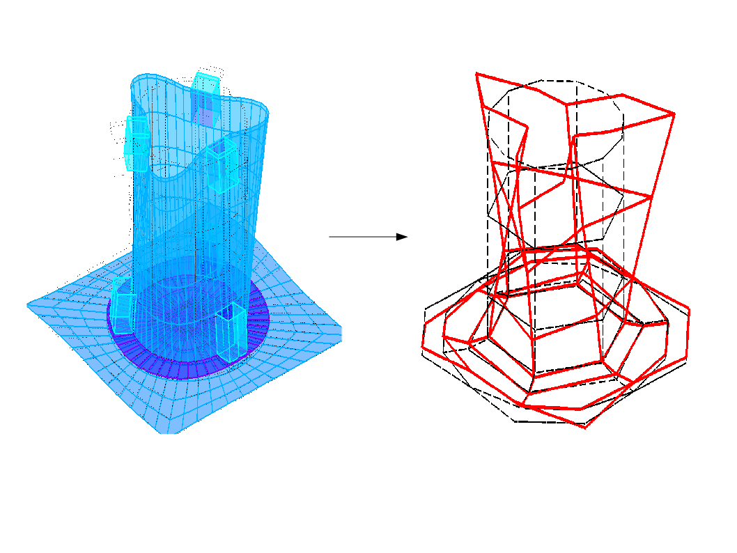
Image 3.2-1 : data projection.
Notes:
Important note: in PROJ_CHAMP, the name of the NUME_DDLdu experimental model must be specified, so that the numberings of the experimental modes and the projected numerical modes are the same.
If NUME_DDLn is not the same, we will not be able to calculate a MAC criterion.
In PROJ_CHAMP, it is necessary to specify the dimension on which we are projecting: by default, we will associate the nodes of the experimental model with 3D elements of the numerical model.
If the numerical model consists of plate elements, it must be specified with CAS =”2.5D”,
If the numerical model is composed of 3D and 2D elements, then it is not possible to specify multiple types of projections. A proposed solution is to assign a plate model (DKTpar example) to the skin elements that cover the 3D elements and to place ourselves in the “2.5D” case.
Operator OBSERVATIONpermet to perform the same operation, with additional options:
use of local references sensor by sensor,
removal of the measured data from the result data structure (for cases where the measurement was made with uniaxial sensors),
creation of a mixed data structure including accelerometric and extensiometric data, to reproduce an accelerometer + gauge measurement,
simulation of a « virtual gauge ».
The description of this operator is provided in the following paragraph.
3.2.2. Using macro command OBSERVATION to project data#
We propose to give a practical example of the use of the macro-command on the following case:
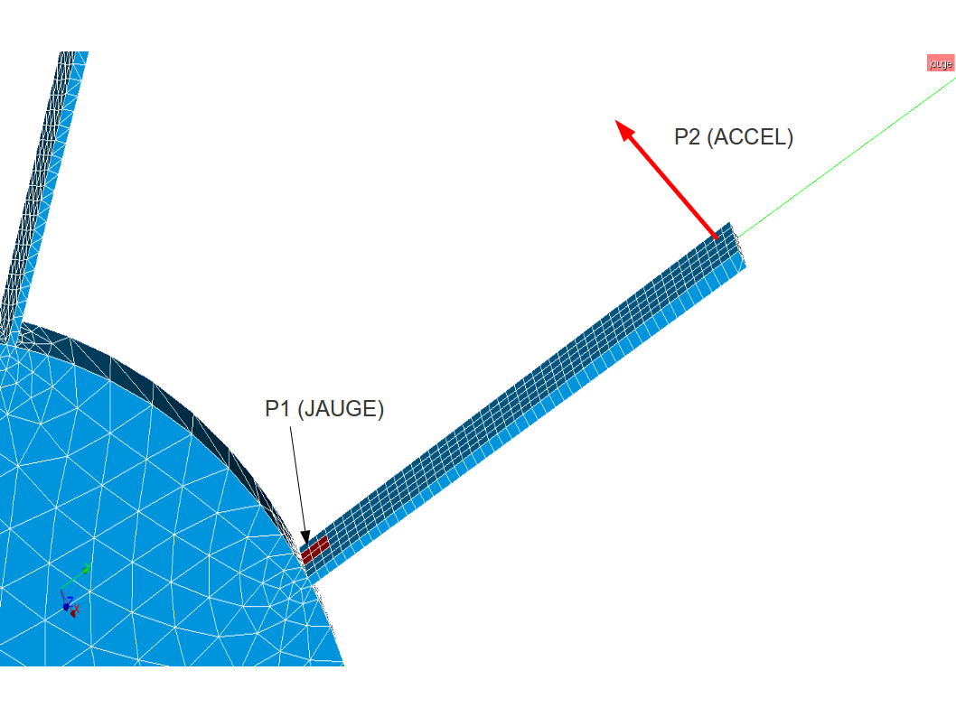
Image 3.2-2 : measurement of the vibrations of a fin using a gauge and an accelerometer.
It is assumed to have measured the vibrations of the bladed wheel represented on the mesh below by placing a gauge at the base of each fin and an accelerometer at the top. The identified specific modes are exported in unv format without going to the global coordinate system. Since the vibrations at the top have only been measured in one direction, we will have a line of the form:
2 4 1 1
2.18331e+01 1.00000e+00 3.74657e-03
1% NOEUD NO1
0.00000e+00 0.00000e+00 7.39432e-01
-1
On node \(\mathit{N01}\), only the local component \(\mathit{DZ}\) was measured. Unmeasured directions are set to 0. In a data set 55, it is not possible to differentiate between unmeasured data and zero measurements.
To compare experimental data and reduced numerical eigenmodes, two operations are required:
on the experimental data, the modes are filtered in order to eliminate the unmeasured data, keeping only one direction for the gauge and the accelerometer
we use OBSERVATIONsans projection (PROJECTION =” NON “), because we’re just filtering the data,
OBSMXT = OBSERVATION (RESULTAT = MESURE,
MODELE_1 = MODMESUR,
MODELE_2 = MODMESUR,
PROJECTION = “NON”,
TOUT_ORDRE = “OUI”,
NOM_CHAM = (“DEPL”, “EPSI_NOEU”,),
FILTRE =( _F (GROUP_NO = “P1”,
NOM_CHAM = “EPSI_NOEU”,
DDL_ACTIF = (“EPXX”,),),
_F (GROUP_NO = “P2”,
NOM_CHAM = “DEPL”,
DDL_ACTIF = (“DZ”,),),),);
on numerical data, the natural modes are projected onto the experimental model:
we use PROJECTION =” OUI “,
we calculate the average deformation for the group of nodes in red in the figure before carrying out the projection: this surface corresponds to the area actually measured by the gauge,
we make the coordinate system changes, using the “NORMALE” option: we calculate the normal to the numerical mesh to define the \(Z\) axis of the local coordinate system (the second axis is defined with the keyword VECT_Y); here, we could also have used the “CYNLINDRIQUE” option.
the components corresponding to the measured data are filtered.
OBSJAU = OBSERVATION (RESULTAT = CALCUL,
MODELE_1 = MODNUME,
MODELE_2 = MODMESUR,
PROJECTION = “OUI”,
TOUT_ORDRE = “OUI”,
NOM_CHAM = “EPSI_NOEU”,
EPSI_MOYENNE = _F (GROUP_MA =” SURF1 “, SEUIL_VARI =( 0.1,),
MASQUE =( “EPYY”, “EPZZ”, “EPXY”,
“EPXZ”, “EPYZ”),),
MODI_REPERE = _F (GROUP_NO = (“P1”, P2”),
REPERE = “NORMALE”,
VECT_Y = (0.,1.,0.)),),
FILTRE =( _F (GROUP_NO = “P1”,
NOM_CHAM = “EPSI_NOEU”,
DDL_ACTIF = (“EPXX”),),
_F (GROUP_NO = “P2”,
NOM_CHAM = “DEPL”,
DDL_ACTIF = (“DZ”,),),),);
3.3. Calculating MAC between two fashion bases#
The calculation of MAC can be done with the MAC_MODES operator, which calculates the matrix of MAC between all the modes of two bases. The data structure produced is a table, which is printed with INFO =2 in MAC_MODES.
The MATR_ASSE keyword allows you to use a weighting matrix.
The printed table has the following form:
ASTER 11.01.03 CONCEPT MAC_ET CALCULE ON 02/15/2012 AT 14:18:54 FROM TYPE
TABLE_SDASTER
MAC! NUME_MODE_1
! 1 2 3 4 5
NUME_MODE_2 1! 1.00000E+00 2.17692E-14 7.49505E-16 5.23742E-22 1.66188E-21
2! 2.17692E-14 1.00000E+00 4.21440E-13 9.40269E-19 1.12652E-19
3! 7.49505E-16 4.21440E-13 1.00000E+00 7.24387E-18 1.28403E-17
4! 5.23742E-22 9.40269E-19 7.24387E-18 1.00000E+00 2.11012E-13
5! 1.66188E-21 1.12652E-19 1.28403E-17 2.11012E-13 1.00000E+00
You can visualize the MAC product in Excel, or use the CALC_ESSAI macro command, which offers a 2D visualization. To do this, launch the macro command without keywords at the end of the calculation, and click on the « model expansion » tab.
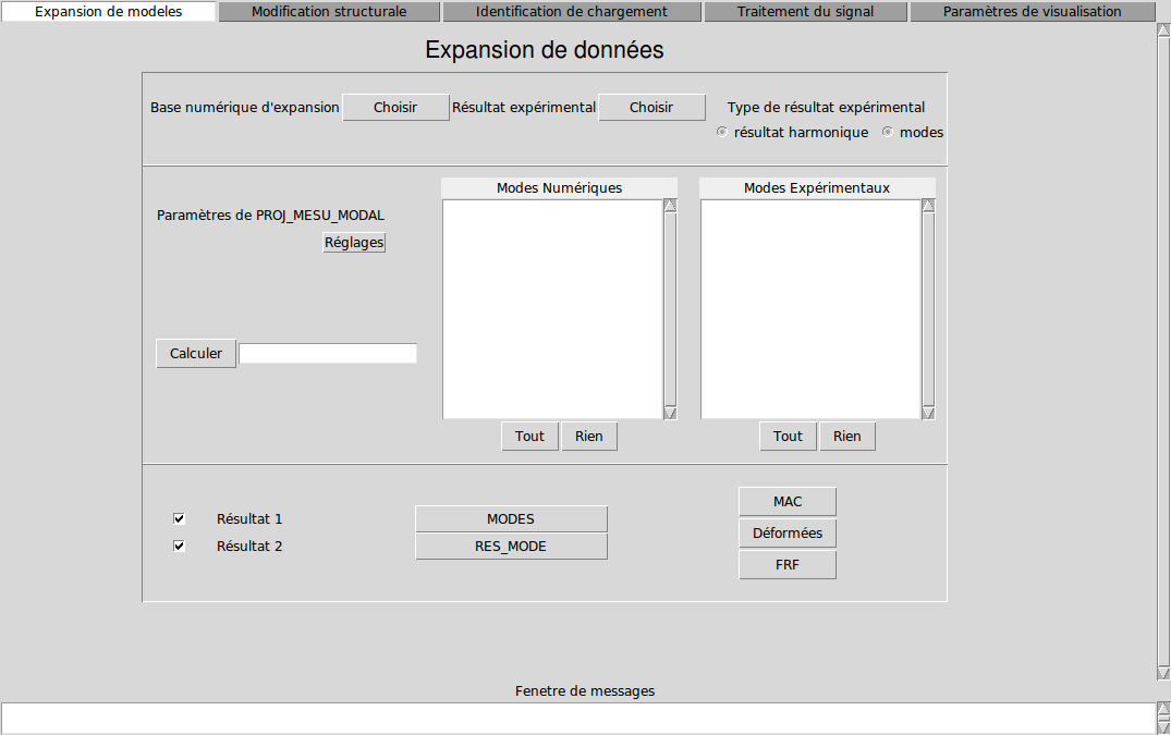
Image 3.3-1 : Image 3.3-1: CALC_ESSAI: model expansion.
In the lower frame, choose the two mode bases to compare (if only one of the two bases is selected, we will do a MAC of the base by itself), and click on MAC. If the selected bases are not defined on the same model, the MAC button is greyed out.
The MAC matrix that appears is as follows:
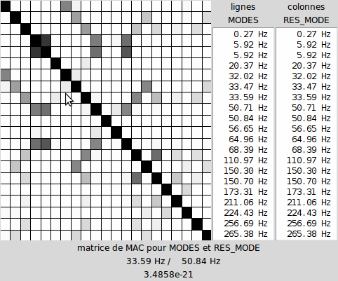
Image 3.3-2 : MAC between two mode bases viewed under CALC_ESSAI.
By passing the mouse over the boxes, you can see at the bottom the frequencies of the modes concerned and the value of MAC for them.
NB: in appendix 5.4, we propose a script using the matplotlib python library to create MAC diagrams in 3D that are more easily interpretable than the one implemented by default in CALC_ESSAI. In the longer term, we are studying the feasibility of integrating the MAC 3D by default with the operator.