5. Appendix#
5.1. Unv mesh data set documentation#
Data set 2411: node description:
Name: Nodes - Double Precision
Status: Current
Owner: Simulation
Revision Date: 23- OCT -1992
Record 1: FORMAT (4I10)
Field 1 – node label
Field 2 – export coordinate system number
Field 3 – displacement coordinate system number
Field 4 – color
Record 2: FORMAT (1P3D25.16)
Fields 1-3 – node coordinates in the part coordinate
System
Records 1 and 2 are repeated for each node in the model.
Exemplo:
-1
2411
121 1 1 11
5.0000000000000000D+00 1.0000000000000000D+00 0.0000000000000000D+00
122 1 1 11
6.000000000
Data set 82: description of connectivities: this data set is no longer used only in very specific cases of experimental meshes. The elements are more generally described by the 2412 data set.
Name: Tracelines
Status: Obsolete
Owner: Simulation
Revision Date: 27-Aug-1987
Additional Comments: This dataset is written by I- DEAS Test.
Record 1: FORMAT (3I10)
Field 1 - trace line number
Field 2 - number of nodes defining trace line
(maximum of 250)
Field 3 - color
Record 2: FORMAT (80A1)
Field 1 - Identification line
Record 3: FORMAT (8I10)
Field 1 - nodes defining trace line
= > 0 draw line to node
= 0 move to node (a move to the first
node is implied)
Notes: 1) MODAL - PLUS node numbers must not exceed 8000.
Identification line may not be blank.
Systan only uses the first 60 characters of the
text identification.
MODAL - PLUS does not support trace lines longer than
125 knots.
Supertab only uses the first 40 characters of the
Identification line for a name.
Repeat Datasets for each Trace_Line
Data set 2412: description of elements (classic EF model) :
Name: Elements
Status: Current
Owner: Simulation
Revision Date: 14- AUG -1992
Record 1: FORMAT (6I10)
Field 1 – label element
Field 2 – fe descriptor id
Field 3 – physical property table number
Field 4 – material property table number
Field 5 – color
Field 6 – number of nodes on element
Record 2: *FOR NON - BEAM ELEMENTS*
FORMAT (8I10)
Fields 1-n – node labels defining element
Record 2: *FOR BEAM ELEMENTS ONLY*
FORMAT (3I10)
Field 1 – beam orientation node number
Field 2 – beam fore-end cross section number
Field 3 – Beam Aft-End Cross Section Number
Record 3: *FOR BEAM ELEMENTS ONLY*
FORMAT (8I10)
Fields 1-n – node labels defining element
Records 1 and 2 are repeated for each non-beam element in the model.
Records 1 - 3 are repeated for each beam element in the model.
Exemplo:
-1
2412
1 11 1 5380 7 2
0 1 1
1 2
2 21 2 5380 7 2
0 1 1
3 4
3 22 3 5380 7 2
0 1 2
5 6
6 91 6 5380 7 3
11 18 12
9 95 6 5380 7 8
22 25 29 30 31 26 24 23
14 136 8 0 7 2
53 54
36 116 16 5380 7 20
152 159 168 167 166 158 150 151
154 170 169 153 157 157 161 173 172
171 160 155 156
-1
5.2. Data set reference material 58#
Number: 58
Name: Function at Nodal DOF
Status: Current
Owner: Test
Revision Date: 23-Apr-1993
Record 1: Format (80A1)
Field 1 - ID Line 1
NOTE
ID Line 1 is generally used for the function
description.
Record 2: Format (80A1)
Field 1 - ID Line 2
Record 3: Format (80A1)
Field 1 - ID Line 3
NOTE
ID Line 3 is generally used to identify when the
function was created. The Date Is In The Form
DD- MMM -YY, and the time is in the form HH:MM:SS,
with a general format (9A1,1X,8A1).
Record 4: Format (80A1)
Field 1 - ID Line 4
Record 5: Format (80A1)
Field 1 - ID Line 5
Record 6: Format (2 (I5, I10), 2 (1X,10A1, I10, I4))
DOF Identification
Field 1 - Function Type
0 - General or Unknown
1 - Time Response
2 - Auto Spectrum
3 - Cross Spectrum
4 - Frequency Response Function
5 - Transmissibility
6 - Coherence
7 - Auto Correlation
8 - Cross Correlation
9 - Power Spectral Density (PSD)
10 - Energy Spectral Density (ESD)
11 - Probability Density Function
12 - Spectrum
13 - Cumulative Frequency Distribution
14 - Peaks Valley
15 - Stress/Cycles
16 - Strain/Cycles
17 - Orbit
18 - Mode Indicator Function
19 - Force Pattern
20 - Partial Power
21 - Partial Coherence
22 - Eigenvalue
23 - Eigenvector
24 - Shock Response Spectrum
25 - Finite Impulse Response Filter
26 - Multiple Coherence
27 - Order Function
Field 2 - Function Identification Number
Field 3 - Version Number, or Sequence Number
Field 4 - Load Case Identification Number
0 - Single Point Excitation
Field 5 - Response Entity Name ( » NONE « if unused)
Field 6 - Response Node
Field 7 - Response Direction
0 - Scalar
1 - +X Translation 4 - +X Rotation
-1 - -X Translation -4 - -X Rotation
2 - +Y Translation 5 - +Y Rotation
-2 - -Y Translation -5 - -Y Rotation
3 - +Z Translation 6 - +Z Rotation
-3 - -Z Translation -6 - -Z Rotation
Field 8 - Reference Entity Name ( » NONE « if unused)
Field 9 - Reference Node
Field 10 - Reference Direction (same as field 7)
NOTE
Fields 8, 9, and 10 are only relevant if field 4
Is zero.
Record 7: Format (3I10,3E13.5)
Data Form
Field 1 - Ordinate Data Type
2 - real, single precision
4 - real, double precision
5 - complex, single precision
6 - complex, double precision
Field 2 - Number of data pairs for uneven abscissa
Spacing, or Number of Data Values for Even
Abscissa spacing
Field 3 - Abscissa Spacing
0 - uneven
1 - even (no abscissa values stored)
Field 4 - Minimum abscissa (0.0 if spacing uneven)
Field 5 - Abscissa increment (0.0 if spacing uneven)
Field 6 - Z-axis value (0.0 if unused)
Record 8: Format (I10,3I5,2 (1X,20A1))
Abscissa Data Characteristics
Field 1 - Specific Data Type
0 - unknown
1 - general
2 - stress
3 - strain
5 - temperature
6 - heat flow
8 - displacement
9 - reaction force
11 - Velocity
12 - acceleration
13 - excitation force
15 - pressure
16 - mass
17 - Time
18 - frequency
19 - rpm
20 - order
Field 2 - Length units exponent
Field 3 - Force units exponent
Field 4 - Temperature units exponent
NOTE
Fields 2, 3 and 4 are relevant only if the
Specific Data Type is General, or in the case of
Computers, the response/reference direction is a
Scalar, or the functions are being used for
Nonlinear connectors in System Dynamics Analysis.
See Addendum “A” for the units exponent table.
Field 5 - Axis label ( » NONE « if not used)
Field 6 - Axis units label ( » NONE « if not used)
NOTE
If Fields 5 and 6 Are Supplied, They Take
Precendence over program generated labels and
units.
Record 9: Format (I10,3I5,2 (1X,20A1))
Ordinate (or ordinate numerator) Data Characteristics
Record 10: Format (I10,3I5,2 (1X,20A1))
Ordinate Denominator Data Characteristics
Record 11: Format (I10,3I5,2 (1X,20A1))
Z-axis Data Characteristics
NOTE
Records 9, 10, and 11 are always included and
Have fields the same as record 8. If Records 10
And 11 are not used, set field 1 to zero.
Record 12:
Data Values
Ordinate Abscissa
Case Type Precision Spacing Format
1 real single even 6E13.5
2 Real Single Uneven 6E13.5
3 complex single even 6E13.5
4 complex single uneven 6E13.5
5 real double even 4E20.12
6 Real Double Uneven 2 (E13.5, E20.12)
7 complex double even 4E20.12
8 complex double uneven E13.5,2E20.12
NOTE
See Addendum “B” for typical FORTRAN READ/WRITE
Statements for each case.
General notes:
ID lines may not be blank. If no information is required,
The word « NONE » must appear in columns 1 through 4.
ID line 1 appears on plots in Finite Element Modeling and is
used as the function description in System Dynamics Analysis.
Dataloaders use the following ID line conventions
ID Line 1 - Model Identification
ID Line 2 - Run Identification
ID Line 3 - Run Date and Time
ID Line 4 - Load Case Name
Coordinates codes from MODAL - PLUS and MODALX are decoded into
node and direction.
Entity names used in System Dynamics Analysis prior to I- DEAS
Level 5 has a maximum of 4 characters. Beginning with Level 5,
Entity names will be ignored if this dataset is preceded by
Dataset 259. If no dataset 259 precedes this dataset, then the
Entity name will be assumed to exist in model bin number 1.
Record 10 is ignored by System Dynamics Analysis unless load
box = 0. Record 11 is always ignored by System Dynamics
Analysis.
In record 6, if the response or reference names are « NONE »
And are not overridden by a dataset 259, but the correspond-
ING node is non-zero, System Dynamics Analysis adds the node
And direction to the function description if space is sufficient
ID line 1 appears on XY plots in Test Data Analysis along
with ID line 5 if it is defined. If Defined, the Axis Units
Labels Also Appear on the XY Plot Instead of the Normal
Labelling based on the data type of the function.
For functions used with nonlinear connectors in System
Dynamics Analysis, the following requirements must be
adhered to:
Record 6: For a displacement-dependent function, the
Function type must be 0; for a frequency-dependent
Function, it must be 4. In either case, the load case
Identification number must be 0.
Record 8: For a displacement-dependent function, the
Specific Data Type Must Be 8 and the Length Units
Exponent must be 0 or 1; for a frequency-dependent
Function, the specific data type must be 18 and the
length units exponent must be 0. In either case, the
Other units exponents must be 0.
Record 9: The specific data type must be 13. The
Temperature units exponent must be 0. For an ordinate
Numerator of force, the length and force units
Exponents must be 0 and 1, respectively. For an
Computer Numerator of Moment, The Length and Force
units exponents must be 1 and 1, respectively.
Record 10: The specific data type must be 8 for
Stiffness and hysteretic damping; it must be 11
For viscous camping. For an ordinate denominator of
Translational Displacement, the Length Units Exponent
Must be 1; for a rotational displacement, it must
Be 0. The other exponents units must be 0.
Dataset 217 must precede each function in order to
Define the function’s usage (i.e. stiffness, viscous
damping, hysteretic damping).
5.3. Data set 55 reference material#
Name: Data at Nodes
Status: Obsolete
Owner: Simulation
Revision Date: 07-Mar-1997
Additional Comments: This dataset is written and read by I- DEAS Test.
RECORD 1: Format (40A2)
FIELD 1: ID Line 1
RECORD 2: Format (40A2)
FIELD 1: ID Line 2
RECORD 3: Format (40A2)
FIELD 1: ID Line 3
RECORD 4: Format (40A2)
FIELD 1: ID Line 4
RECORD 5: Format (40A2)
FIELD 1: ID Line 5
RECORD 6: Size (6I10)
Data Definition Parameters
FIELD 1: Model Type
0: Unknown
1: Structural
2: Heat Transfer
3: Fluid Flow
FIELD 2: Analysis Type
0: Unknown
1: Static
2: Normal Mode
3: Complex eigenvalue first order
4: Transient
5: Frequency Response
6: Buckling
7: Complex eigenvalue second order
FIELD 3: Data Characteristic
0: Unknown
1: Scalar
2:3 DOF Global Translation
Vector
3:6 DOF Global Translation
& Rotation Vector
4: Symmetric Global Tensor
5: General Global Tensor
FIELD 4: Specific Data Type
0: Unknown
1: General
2: Stress
3: Strain (Engineering)
4: Element Force
5: Temperature
6: Heat Flux
7: Strain Energy
8: Displacement
9: Reaction Force
10: Kinetic Energy
11: Velocity
12: Acceleration
13: Strain Energy Density
14: Kinetic Energy Density
15: Hydro-Static Pressure
16: Heat Gradient
17: Code Checking Value
18: Coefficient Of Pressure
FIELD 5: Data Type
2: Real
5: Complex
FIELD 6: Number Of Data Values Per Node (NDV)
Records 7 And 8 Are Analysis Type Specific
General Form
RECORD 7: Size (8I10)
FIELD 1: Number Of Integer Data Values
1 < Gold = Nint < Gold = 10
FIELD 2: Number Of Real Data Values
1 < Gold = Nerval < Gold = 12
FIELDS 3-N: Type Specific Integer Parameters
RECORD 8: Size (6E13.5)
FIELDS 1-N: Type Specific Real Parameters
For Analysis Type = 0, Unknown
RECORD 7:
FIELD 1:1
FIELD 2:1
FIELD 3: ID Number
RECORD 8:
FIELD 1:0.0
For Analysis Type = 1, Static
RECORD 7:
FIELD 1:1
FIELD 2:1
FIELD 3: Load Case Number
RECORD 8:
FIELD 11:0.0
For Analysis Type = 2, Normal Mode
RECORD 7:
FIELD 1:2
FIELD 2:4
FIELD 3: Load Case Number
FIELD 4: Number mode
RECORD 8:
FIELD 1: Frequency (Hz)
FIELD 2: Modal Mass
FIELD 3: Modal Viscous Damping Ratio
FIELD 4: Modal Hysteretic Damping Ratio
For Analysis Type = 3, Complex Eigenvalue
RECORD 7:
FIELD 1:2
FIELD 2:6
FIELD 3: Load Case Number
FIELD 4: Number mode
RECORD 8:
FIELD 1: Real Part Eigenvalue
FIELD 2: Imaginary Part Eigenvalue
FIELD 3: Real Part Of Modal A
FIELD 4: Imaginary Part Of Modal A
FIELD 5: Real Part Of Modal B
FIELD 6: Imaginary Part Of Modal B
For Analysis Type = 4, Transient
RECORD 7:
FIELD 1:2
FIELD 2:1
FIELD 3: Load Case Number
FIELD 4: Time Step Number
RECORD 8:
FIELD 1: Time (Seconds)
For Analysis Type = 5, Frequency Response
RECORD 7:
FIELD 1:2
FIELD 2:1
FIELD 3: Load Case Number
FIELD 4: Frequency Step Number
RECORD 8:
FIELD 1: Frequency (Hz)
For Analysis Type = 6, Buckling
RECORD 7:
FIELD 1:1
FIELD 2:1
FIELD 3: Load Case Number
RECORD 8:
FIELD 1: Eigenvalue
RECORD 9: Format (I10)
FIELD 1: Node Number
RECORD 10: Size (6E13.5)
FIELDS 1-N: Data At This Node (NDV Real Or
Complex Values)
Records 9 And 10 Are Repeated For Each Node.
5.4. Script for the 3D representation of a MAC diagram#
This script can be copied at the bottom of a command file, by replacing the names \(\mathit{B1}\) and \(\mathit{B2}\) on the last line with the names of the two databases that you want to compare with MAC.
Warning: this script is based on the matplotlib library that must be installed.
def mac_plot_lib (BASE1, BASE2):
« « » calculates the mac between two bases, extracts it and represents it in a 3d graph
matplotlib » « «
BASE_2 = BASE2);
mactmp=__ MAC. EXTR_TABLE ()
mac = mactmp [“NUME_MODE_1”, “NUME_MODE_2”, “”, “MAC”] .Cross ()
mac_py = mac.values ()
Import numpy as nP
from mpl_toolkits.mplot3d import axes3d
import matplotlib.pyplot as plt
freq_1 = BASE1. LIST_PARA () [“FREQ”]
freq_2 = BASE2. LIST_PARA () [“FREQ”]
order_number_1 = BASE1. LIST_PARA () [“NUME_ORDRE”]
order_number_2 = BASE2. LIST_PARA () [“NUME_ORDRE”]
nb_freq_1 = len (freq_1)
nb_freq_2 = len (freq_2)
matrice_mac = np.transpose (np.array ([mac_py [kk] for kk in number_order_1]))
fig = plt.figure ()
ax = axes3d.axes3d (fig)
# Create regular mesh from coordinates
xpos, ypos = np.meshgrid (np.arange (nb_freq_1), range (nb_freq_2))
xpos = xpos + 0.5* (np.ones (matrice_mac.shape) -matrice_mac)
ypos = ypos + 0.5* (np.ones (matrice_mac.shape) -matrice_mac)
xpos = xpos.flatten ()
ypos = ypos.flatten ()
dx=matrice_mac.flatten ()
dy = dx.copy ()
dz = dx.copy ()
zpos=np.zeros (nb_freq_1*nb_freq_2)
for kk in range (len (xpos)):
if xx [kk] <1.0E-6:
# to avoid crashes in case of a Mac that is too small
xx [kk] =dy [kk] =dz [kk] =1.0E-6
ax.bar3d (xpos [kk], ypos [kk], zpos [kk],
xx [kk], dy [kk], dz [kk],
color=mac2col (dz [kk]))
ax.set_xlabel (u” FREQ_I “)
ax.set_ylabel (u” FREQ_J “)
ax.set_zlabel (u” MAC “)
plt.show ()
def mac2col (value):
# gives the value of the color corresponding to a value of MAC
# between 0 and 1
import matplotlib.colors as colors
import matplotlib.com as CMS
value = 1-value
desc=cm.rdylbu. _segmentdata
segments= [desc [“blue”] [kk] [0] for kk in range (len (desc [“blue”]))))]
num_seg=0
for kk in segments:
if value > kk:
num_seg = num_seg+1
sort =( desc [“red”] [num_seg] [1],
desc [“green”] [num_seg] [1],
desc [“blue”] [num_seg] [1])
return colors.rgb2hex (sort)
mac_plot_lib (B1, B2)
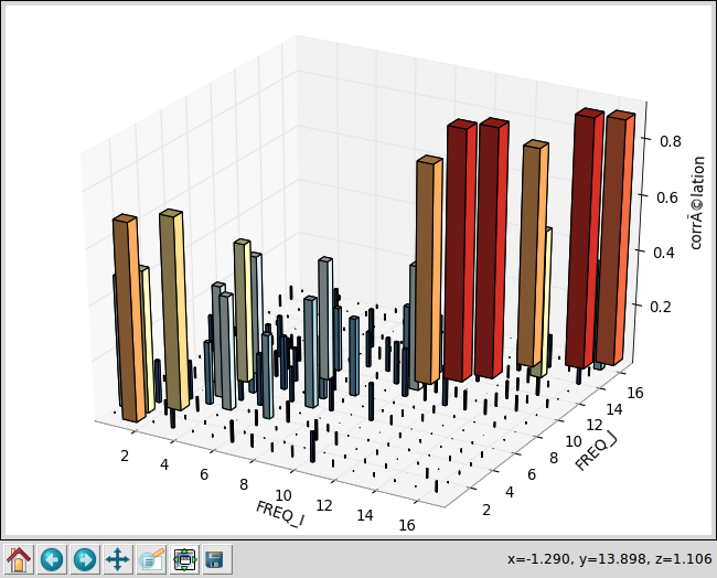
Picture 5.4-1 : MAC 3D.