3. Discretization of the ongoing problem

In addition to the advice previously given for the continuous model, this chapter will list the most important aspects to respect in order to obtain a discretized model adapted to [DYNA_NON_LINE].

3.1. Meshing

As a prerequisite for the transitory calculation, it is strongly recommended to conduct a modal calculation (with [CALC_MODES]), in order to obtain modal information that will make it possible to qualify the quality of the model in dynamics and to adjust certain parameters. Since the objective is not to go into the details of modal analysis, we can nevertheless recall a few rules.

In general, we can define a cutoff frequency for the problem to be studied, and therefore an associated modal truncation. The good representation of all the modes in this truncated base can give information on the mesh sizes to be used, in addition to the considerations already taken into account for quasistatic calculations. Broadly speaking, about ten meshes per smallest wavelength is sufficient (to be adjusted according to the richness of the elements, of course).

Modal analysis will also make it possible to verify that the model is free of problems such as undefined contributions to inertia or stiffness.

Finally, it is essential for the use of modal damping in DYNA_NON_LINE or for adjusting Rayleigh damping, as we will see in the following (cf. Depreciation modeling).

In a much more pronounced way than for quasistatic calculations, dynamic resolution will not accommodate meshes with sudden variations in element sizes. Indeed, these zones can be assimilated to interfaces that will disturb the propagation of waves. We can then see reflected waves appear that are superimposed on « physical » wave trains. Likewise, if we want a good representation of waves, the mesh must be fine along the entire path of the waves: we can only refine in certain non-linear areas. If a wave starts from a finely meshed zone to go to a coarser meshed zone, it will undergo a filter and the wave reflected by the opposite edge risks being strongly disturbed, or even disappearing. If we are only interested in short durations, therefore before any wave feedback on the finely meshed zone, then this error on the reflected wave is not a disadvantageous step. On the other hand, if we want to calculate solutions over longer periods of time, the error committed may be significant.

Finally, unlike the quasistatic case, time has a physical meaning and the time scales that we want to analyze are strongly coupled to the spatial scales of the discretized problem. Thus, the time step is linked to the mesh size, which can be immediately perceived with the concept of stability condition CFL for explicit diagrams.

3.2. Time integration diagram

Since time has a physical meaning in dynamics, the quality of its discretization is all the more sensitive. The role of an integration diagram is to express by an approximate expression two relationships between the quantities (« DEPL », « VITE », « ACCE ») at the previous moment and those at the next moment. The equations of motion are the third set of equations that allows you to close the system to be solved. Depending on the main quantity (« DEPL », « VITE », « « , « ACCE ») that we choose as a pilot to express these equations we adopt a type of « FORMULATION »: « DEPLACEMENT », « « , « VITESSE », « ACCELERATION ».

Some rules for choosing a time step can be set out:

• the evolution of the imposed loads must be sampled in a sufficiently fine manner (between 5 to 10 time steps per shortest period of the signals in question),

• the modal behavior of the structure must be well represented (as above, we must have between 5 and 10 time steps per period of the lowest of the modes considered up to the cutoff frequency), in particular, the frequency distortion caused by the time integration scheme must be limited: the choice of taking between 5 and 10 time steps per period the lowest of the modes considered up to the cutoff frequency ensures a frequency distortion of less than one percent.

Given the low frequency, at best medium frequency, nature of most of the problems that can be addressed here, these two rules are generally not very penalizing.

The choice of the temporal integration scheme and its parameters is made with the keyword factor: « SCHEMA_TEMPS =_F (…) ».

Test cases SDLD31 [V2.01.031] and SDLD32 [V2.01.032] offer a comparison of the temporal integration schemes proposed in DYNA_NON_LINE and in [DYNA_VIBRA] on simple linear systems under harmonic excitation.

3.2.1. Explicit integration diagram

With an explicit, conditionally stable integration scheme dedicated to the problems of « fast dynamics » in the presence of transients with « high frequency » content, it is also necessary to respect the current stability condition (known as « CFL » cf. [R5.05.05] and Bibliography) under penalty of numerical divergence (« explosion » of kinetic energy). In Code_Aster, these schemes are treated in « FORMULATION =” ACCELERATION “(we want to solve by inverting the mass matrix). The mass matrix, which must be invertible, is preferably chosen in diagonal form (*lumpee*) for performance reasons; this is obtained by the keyword: "MASS_DIAG = 'OUI '. The lumpee mass matrix makes it possible to correct part of the frequency drift over long periods of time resulting from the time error induced by the integration diagram. For structural elements, for example DKT/DKTG/DST, it is necessary to specify in AFFE_CARA_ELEM, under the keyword factor « COQUE », the simple keyword « INER_ROTA = “OUI “ », in order to have non-zero inertia terms along the entire diagonal of the mass matrix, even if they are low, in order to have non-zero inertia terms along the entire diagonal of the mass matrix, even if they are low, [R3.07.03].

However, since this option is not available for all finite elements, or with all discrete elements, it is then necessary to solve with the consistent mass matrix, as if implicitly. For HM modeling elements, the mass matrix has zero terms for some specific degrees of freedom, for example pressure. In this case too, one must solve with the consistent mass matrix, to which one adds a small contribution from the stiffness matrix with the keyword « COEF_MASS_SHIFT ».

Two explicit diagrams are available:

• centered differences (« DIFF_CENT ») which is non-dissipative,

• Tchamwa-Wielgosz (« TCHAMWA ») which is dissipative, in a manner comparable to HHT.

It is recommended to start by using a non-dissipative scheme.

The automatic calculation of the Current condition on a modal basis is accurate and will always be valid regardless of the type of finite element used.

For the explicit integration scheme of centered differences « DIFF_CENT », the critical time step is \(2/{\omega}_{max}\) with \({\omega}_{max}\) which is the highest natural pulsation of the discretized system. The presence of shock stiffness associated with the penalized modeling of frictional or non-friction contact significantly increases this higher natural pulsation. In the presence of physical damping (reduced damping coefficient \(\xi\)), the critical time step has the expression: \(2 \left(\sqrt{1+\xi^2}-\xi\right)/{\omega}_{max}\).

We can calculate this pulsation with « CALC_MODES » by choosing the option ``”PLUS_GRANDE “``(or with the option « PLUS_PETITE » by inverting the roles of the mass and stiffness matrix).

For the Tchamwa-Wielgosz dissipative explicit integration scheme “TCHAMWA” (see [bib11] _), the critical time step is slightly lower than that of the « DIFF_CENT » diagram and decreases when the numerical damping linked to the schema is increased (parameter « PHI », whose default value is \(1.05\)).

The current stability condition can also be approximated, at least on models with massive finite elements, by \(\Delta t={l}_{\mathrm{min}}/c\) with \({l}_{\mathrm{min}}\) which is the smallest length of the discretized model and \(c\) the speed of the traction waves at the point in question.

The operator « DYNA_NON_LINE » uses this formula to approximate the stability condition of Current. However, there are some limitations:

1. we do not know how to automatically calculate the current stability condition associated with the presence of discrete springs (this is not programmed),

2. the formula for structural elements (shells, plates and beams) is not corrected.

Therefore, there may be cases where the returned value is not a step below the true Current condition. Therefore, in case of discrepancy, the time step should be shortened.

In addition, the calculation of the current stability condition is not updated and is done only at the beginning of the calculation, based on the speed of the elastic waves for the initial state. If the elastic modulus decreases (damage), the initial current stability condition may become too severe. There is no risk of divergence (except for materials whose elastic modulus could increase), but time CPU could be reduced a bit by updating the Courant stability condition (as is done in codes dedicated to fast dynamics, such as Europlexus [bib2] _).

For most structures, the current stability condition is very penalizing: the speed of the waves is often of the order of a few thousand \(m\mathrm{/}s\), we arrive at time steps of less than \({10}^{\mathrm{-}5}s\), for finite element dimensions chosen for usual structures. This therefore requires a very high total number of moments to describe the transient, so it produces a considerable volume of results.

If one solves the problem on a reduced modal basis (keyword factor « PROJ_MODAL =_F () »), then the disadvantage of the very low critical time step for an explicit schema disappears. In fact, the time limit step will be directly proportional to the smallest specific period of the truncated modal base. We have the relationship: \(\Delta t=2/\omega\) with \(\omega\) which is the highest natural pulsation in the system. The more truncated the modal base is, the greater the associated critical time step will be.

In addition, the calculation of the Current condition is then immediate because we explicitly know all the pulsations of the base, and therefore the highest in particular.

With an explicit diagram, it is recommended to place yourself slightly below the Current condition: between 0.5 and 0.7 times the Current Stability condition. There will be no sub-division of the time step due to non-convergence at the global balance scale: the user remains solely in control of the time step throughout the calculation. On the other hand, via the keyword factor COMPORTEMENT, cf. [U4.51.11], the user indicates his requirements for the integration of the law of nonlinear behavior, which can lead to the automatic division defined in the command [DEFI_LIST_INST].

notes

• if boundary conditions are imposed on the move that change over time, it must be taken into account that these conditions are in fact being imposed at an accelerated pace explicitly (because it is the primal unknown). This means that one has to enter « DYNA_NON_LINE » the second derivative of the moving signal that you want to impose. This evolution of the imposed displacement must therefore be differentiable at least twice in time.

• The use of quadratic elements is not explicitly recommended: in fact, parasitic oscillations may appear on the solution fields (displacement or constraints). This phenomenon can also be amplified by the joint use of consistent mass matrix

• For the verification of the hypothesis of plane stresses, if we use the de Borst method, the associated global iterative process is then stuck at the first iteration (unlike the implicit case). This may result in a slight imprecision of the results, tempered by the fact that the time step being otherwise very small, the non-flatness of the stresses can only be very moderate. However, it is entirely possible to use the local version of the de Borst algorithm through the keyword « ITER_CPLAN_MAXI » under the keyword factor « COMPORTEMENT », see [Comportements non-linéaires]. Indeed, these local iterations take place explicitly, with an associated additional calculation cost.

3.2.2. Implicit integration diagram

With an implicit integration scheme, which makes it possible to best respect the conditions of non-linear dynamic equilibrium, dedicated to the problems of « slow dynamics » in the presence of transients with « low frequency » content, in a phase of developing the transient simulation, it is recommended to compare the results obtained for two choices of time step values. Implicitly, the proposed schemes are unconditionally stable, but that does not mean that we can take any step of time! A step too big will not lead to a discrepancy, but the error in the solution, such as frequency distortion, will obviously be significant.

These schemas can be accessed in « FORMULATION = » DEPLACEMENT « « , « ," FORMULATION =" VITESSE "", "FORMULATION =" ACCELERATION ". The « FORMULATION = » DEPLACEMENT «  » « is completely natural and preferred in the case of material non-linearities, because the internal forces result from the treatment of the behavioral relationship expressed from the deformations themselves obtained with the displacement field. It is not possible to use a lumpee mass matrix with these diagrams.

It is recommended to ensure a uniform and regular sampling of the time step whenever possible. However, in the presence of behavioral nonlinearities, it is not possible or desirable to avoid temporal redistribution in the event of non-convergence of the Newton algorithm, driven by the step subdivision directives that will have been defined in the command [DEFI_LIST_INST].

Implicit schemas can be classified into two categories:

• average acceleration (« NEWMARK ») of order 2 and which does not provide numerical dissipation: to be used first,

• HHT complete (« MODI_EQUI = “OUI “, option by default) which remains of order 2, unlike the case of the modified average acceleration. If more damping is desired at medium frequency, then the modified mean acceleration scheme can be used with "MODI_EQUI = 'NON ', and the pattern becomes of order 1. The complete HHT scheme (« MODI_EQUI = “OUI “ ») is specifically developed to introduce high-frequency digital damping and therefore not to disturb the low-frequency physical response. Damping is directly controlled by the parameter ALPHA of the diagram,

If we observe high frequency oscillations in the numerical solution (basically, oscillations whose period is of the order of a few steps of time), we will prefer to choose the complete HHT diagram, to start with a value of the order of \(–\mathrm{0,1}\) for the parameter « ALPHA ». A value of \(–\mathrm{0,3}\) is a high limit that can still be used. It is strongly recommended to conduct a parametric study on the value of the parameter « ALPHA » in order to choose the value closest to zero that allows a correct solution to be obtained without numerical overdamping.

Refer to paragraph §5.4 of [R5.05.05].

Implicit schemas should be used, first of all, with a displacement formulation: « FORMULATION = “DEPLACEMENT “``.

3.2.3. Summary for the choice of the integration scheme

The following table summarizes the key points.

Finally, it should be noted that the analytical results on the characteristics (convergence, frequency distortion, error, numerical damping, overshooting…) of time patterns are obtained for a linear framework. Demonstrations in a non-linear regime are very rare and are limited to specific cases. In practice, some characteristics of the diagrams may degrade to non-linear. This may explain why it is not necessarily essential to use the diagram which, in linear mode, will have exceptional performances (order 4…), but that it is better to prefer simpler and more robust schemes, in particular with high frequency digital dissipation.

Likewise, in non-linear mode, the precise evaluation of the current stability condition of an explicit diagram requires an update of its calculation. Indeed, the current stability condition calculated initially may not be conservative (for example if some elements see their size decrease, or if shocks occur, with modeling by penalization). This calculation is not updated and in case of discrepancy, it is recommended to reduce the time step and to restart the calculation.

However, the results of linear analysis on the diagrams constitute a solid basis for their analysis (cf. [R5.05.05] and Bibliography), while knowing that non-linearities can disturb the behavior of the diagrams.

The time step to be imposed can be wisely limited:

• in higher value, by the time step to be respected in order to properly discretize the changes in imposed loads and to properly represent the highest natural frequency of the system that one wants to take into account,

• in a lower value, by the stability condition of Courant, in the sense that it has the shortest time for which information can pass from one node in the mesh to another.

Between these boundaries, it is essential to conduct a parametric study to ensure the correct convergence of the digital solution.

The lower bound gives crucial information about the maximum subdivisions of the time step that should be allowed when the algorithm does not converge. Allowing the time step to be subdivided until it reaches clearly under the current stability condition may be useless because the calculated solution is then likely to suffer numerical pollution that will not facilitate convergence.

Still in connection with the iterations to check the balance at each step, it can be noted that, in most cases, if the time step is sufficiently fine, the maximum number of convergence iterations remains moderate: often of the order of 10, while in quasistatic, it is common to exceed these values.

So the idea is to say that the time step is a good order of magnitude if the number of convergence iterations remains moderate. If this number increases, one can try to reduce the step slightly, always respecting the limits defined above. However, there are cases where you may, from time to time, need to allow more iterations during a few steps.

Finally, if you are forced to change the schema from time to time to use a dissipative schema, like HHT, it is essential to conduct a parametric study on this damping. Indeed, the risk of introducing too great a dissipation is not negligible, especially with the modified mean acceleration pattern. The next paragraph will return to this point.

3.3. Initial conditions

We will favor regular initial conditions: displacements and velocities differentiable in \(t=t_0\), state of constraints in equilibrium at \(t=t_0\) for example resulting from a quasistatic calculation with [STAT_NON_LINE]. Indeed, many time schemes evaluate a predictor of the initial acceleration from the initial state, by inverting the mass matrix (if it is feasible): if this initial acceleration is excessive, the disturbance can propagate over the transient, especially if the damping is low and generate parasitic oscillations in the solution (« overshooting »). If the mass matrix is not invertible, see section Modifying the mass matrix.

3.4. Depreciation modeling

The order of introduction and use of dissipation in discretized finite element modeling of a structure is as follows:

1. intrinsic dissipation linked to the irreversible non-linear behavior relationships of the constituent materials affected on the support cells of finite elements, cf. keyword factor « COMPORTEMENT =_F (RELATION =”… “) ``cf. [Comportements Non Linéaires]. These behavior models can dissipate energy during deformation-stress cycles (for example in elastoplasticity) and/or in deformation-stress rates (for example in nonlinear viscoelasticity, in viscoplasticity),

2. intrinsic dissipation linked to irreversible non-linear behavior relationships of bonds on interfaces (collision, friction…): cf. keyword factor « COMPORTEMENT » with relationships: « DIS_CHOC », « DIS_CONTACT », « CHOC_ENDO », « « , « , » « , », « CHOC_ENDO_PENA », using the parameters AMOR_NOR and AMOR_TAN of the corresponding materials, cf. [ R5.03.17] and [AFFE_CARA_ELEM], which dissipate energy during cycles in displacement-force jumps (for example in elastoplasticity) and/or in displacement-force jump speeds. Damping forces proportional to the speed on these interfaces are added to the equations of motion, depending on whether or not the friction contact is activated, without making a contribution to the damping matrix,

3. dissipation related to linear viscous damping assigned to discrete elements, cf. command [AFFE_CARA_ELEM] (keyword factor « DISCRET » or « DISCRET_2D », keyword « CARA = “A_T_D_N”``, etc… ),

4. global dissipation of the structural damping type (Rayleigh or modal, also known as Wilson & Penzien, which can be used simultaneously),

5. dissipation related to absorbent borders (Sommerfeld condition modeled with paraxial elements of order 0) of an elastic domain or a perfect fluid domain (3D_ ABSO ``, ``D_ PLAN_ABSO ", ``3D_ FLUI_ABSO", ``3D_ ", ``3D_", ``3D_ ","", ``3D_ ",, », « « , « « , « « , « , » », « « , « « , « « , « « , « , » », « « , « « , « « , « « , « « , « « , « « , « « , « « , « « , «  » FLUI_ABSO FLUI_ABSO AXIS_FLUI_ABSO R4.02.05

6. numerical dissipation provided by the diagram in time.

Ideally, the first categories should be sufficient, but in practice, for reasons of simplification of the modeling, it is often essential to add structural damping, the damping provided by the diagram in time being the last resort.

We will only discuss here the use of structural damping and the one linked to the temporal integration scheme (for more information on this point, the reader can refer to the documentation [U2.06.03]).

The overall dissipation of the structural damping type is taken into account by modal damping or Rayleigh damping.

The transitional resolution with « DYNA_NON_LINE » uses:

• the global damping matrix combining by summation all the contributions: the global Rayleigh damping: the global Rayleigh damping, the linear viscous damping assigned to discrete elements, the finite elements of absorbent boundaries (paraxial of order 0) solid and fluid, the constant matrix defined for condensed substructures (dynamic macroelements), and the matrix that « DYNA_NON_LINE » assembles from an elementary damping matrix built outside the operator for be able to add (accumulate) possibly damping of another nature, for example « IMPE_MECA » in U-P formulation of perfect fluid-structure interaction. This is the purpose of the optional keyword: « MATR_ELEM_AMOR » to provide it to « DYNA_NON_LINE ». See test case [zzzz420a],

• the vector of viscous forces combining all the contributions: modal damping.

It is possible to use both global Rayleigh damping, as well as modal damping and also numerical damping of the time diagram. In these cases of combinations of several damping sources (not including material dissipation due to the selected behavioral relationship or touch-friction), the user must check the overall coherence of the dissipation and therefore not to risk counting damping several times on the same zone. For example, if you want to combine global damping (Rayleigh or modal) and material dissipation, in general the regulations require lowering the global damping value compared to a purely elastic calculation.

Note, cf. [R4.02.05], that paraxial elements should not be used in the case « MULTI_APPUI ».

Another example: the case of a building with seismic supports. If we want to represent the dissipation of supports by a local model (non-linear law or shock absorbers) and the damping of the building by modal damping, it will be necessary to verify that we are not introducing modal damping on modes that mainly make the supports work, such as horizontal rigid body modes (two translations and vertical axis rotation).

Finally, let’s remember that the more sources of dissipation are multiplied, the more difficult will be their control and their physical interpretation.

3.4.1. Structural amortization

In non-linear transient dynamics, Code_Aster proposes two types of models of this type:

1. modal damping (from Wilson & Penzien), defined uniformly over the entire finite element model, after establishing a reduced modal base over a given representative frequency band, intervening in the form of assembled viscous forces, linear to the speed vector,

2. the global Rayleigh damping, defined according to the allocation of the materials on the mesh, intervening in the form of an assembled matrix performing the linear relationship between the viscous forces and the speed vector.

For a linear system with two degrees of freedom, these two models give the same viscous forces if the Rayleigh damping calibration is performed on the two natural frequencies. In the other cases, the viscous forces differ.

If we solve the equations of the driven coordinate system, by considering a rigid translational training movement, the driving inertia forces being defined with the command [:ref:CALC_CHAR_SEISME<U4.63.01>] (MONO_APPUI = “OUI”), then the damping is constructed with the relative speed vector. We recall that in non-linear dynamics, cf. [R5.05.05], if the movements imposed on the supports are not a rigid body movement (case « MULTI_APPUI »), then we must solve the equations of motion in absolute coordinate system (Galilean).

3.4.1.1. Modal amortization

With regard to modal depreciation, we insist on compliance with the three basic rules:

• check that the associated modal base (« MODE_MECA ») is sufficiently complete (containing at least the entire excitation spectrum) to not have an absence of damping according to certain response modes of the structure,

• check that all the values of the modal damping coefficients (« AMOR_REDUIT / LIST_AMOR ») are positive for all the modes selected (« MODE_MECA »), because any negative value risks causing dynamic instability,

• since modal damping is treated explicitly in « DYNA_NON_LINE » (the viscous forces being expressed with the velocities obtained at the previous step), it may be necessary to decrease the time step so that the integration in time remains stable, even with an implicit pattern in time that is unconditionally stable.

In fact, the assembled amortization matrix is not calculated because it would be full and therefore expensive.

This modal base, used to define modal amortizations, must imperatively have the same numbering profile as that of the dynamic system matrices used when calculating the response itself. Before using the modal depreciations of the modal base in calculating the response, this rule therefore possibly requires the prior transformation of this initial modal base into a new modal base, the definition of the boundary conditions of which is identical to that relating to the calculation of the response with « DYNA_NON_LINE », thus ensuring the same number and the same position of the dualization Lagrange multipliers. This is particularly the case when applying non-zero imposed trips to calculate the response. The zzzz113a test case details the corresponding procedure.

If the structure studied consists of several substructures or sub-domains, composed of specific materials, whose reduced damping coefficients differ, a practice consists in the following evaluation of an equivalent modal damping coefficient (for a given mode) according to the rule of RCC -G 1988, ETC -C 2012 (section 1.A.5.4). This modeling is accessible, cf. [CALC_AMOR_MODAL] (AMOR_INTERNE =_F (…), AMOR_SOL =_F (…),…). Care should be taken not to have shock absorbers provided on discrete elements, at the risk of amortizing twice!

3.4.1.2. Rayleigh damping

This modeling uses a global viscous damping matrix \({\bf C}\) as the assembly on the finite element model of a linear combination of stiffness and mass matrices. This global damping matrix is only diagonalized on the basis of natural eigenmodes if the calibration of the Rayleigh parameters is identical throughout the finite element model. Rayleigh damping parameters are provided by the keyword factor “ELAS” in the [DEFI_MATERIAU] operator.

\[\]

: label: EQ-Amorrayleigh

{bf C} =alpha {bf K} +beta {bf M}

Three identification cases are presented here to illustrate the effects induced by this modeling:

• damping proportional to inertia characteristics: \(\alpha =0\) \(\beta ={\beta }_{i}\).

This case has been widely used in transient resolution in the « ACCELERATION » formulation: if the mass matrix is diagonal, the damping matrix is still diagonal and the gain in memory space is obvious. The coefficient \(\beta\) can be identified with the experimental reduced damping \({\xi }_{i}\) of the eigenmode \(({\rho }_{i},{\omega }_{i})\) which contributes the most to the response, hence \({\beta }_{i}=2{\xi }_{i}{\omega }_{i}\). For any other pulsation a reduced modal damping \(\xi ={\beta }_{i}\frac{{\omega }_{i}}{\omega }\) is obtained. Responses on high order \(\omega \gg {\omega }_{i}\) modes will be very poorly damped and those on low frequency \(\omega <{\omega }_{i}\) modes will be too damped.

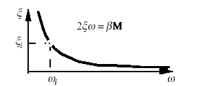
This damping proportional to mass is the only Rayleigh damping that is easily usable with an explicit integration diagram. It is shown in Figure u2.06.13-amorPropMass. Indeed, it can be shown that the introduction of a term proportional to the stiffness leads to a decrease in the critical time step (condition CFL).

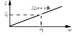
• damping proportional to stiffness characteristics: \(\alpha ={\alpha }_{j}\) \(\beta =0\).

The coefficient can be identified, as before, from the modal damping \({\xi }_{j}\) associated with the \(({\rho }_{j},{\omega }_{j})\) mode, from where \({\alpha }_{j}=2\frac{{\xi }_{j}}{{\omega }_{j}}\). For any other pulsation a reduced modal damping \(\xi ={\alpha }_{j}\frac{\omega }{{\omega }_{j}}\) is obtained. The responses on high modes \(\omega \gg {\omega }_{j}\) are therefore very amortized. It is illustrated in figure u2.06.13-amorPropRigi

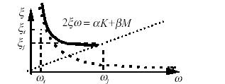
• full proportional damping: \(\alpha ={\alpha }_{j}\) \(\beta ={\beta }_{i}\).

From an identification on two different natural frequencies \(({\rho }_{i},{\omega }_{i})\) and \(({\rho }_{j},{\omega }_{j})\), we will obtain for any other pulsation a reduced modal damping \(\xi ={\alpha }_{j}\frac{\omega }{{\omega }_{j}}+{\beta }_{i}\frac{{\omega }_{i}}{\omega }\). In the interval \([{\omega }_{i},{\omega }_{j}]\) the variation in the reduced damping is low and outside it we find the combination of the previous disadvantages: the responses on the modes outside the interval are too damped.

: name: u2.06.13 - amorProp full

Full Rayleigh damping rate

The complete Rayleigh damping illustrated in FIG. u2.06.13-amorPropComplet makes it possible to have an almost constant damping value on a given frequency plateau, always greater than \(\sqrt{\alpha \beta}\), which makes it possible to control its effect over a frequency range defined in coherence with the problem in question. However, when stiffness is damaged, the transient dynamic responses have a decreasing central frequency. The perceived Rayleigh damping is then slightly stronger at low frequencies and weaker at high frequencies.

Application to the structure

The Rayleigh global viscous damping coefficients are defined, at the level of material characteristics (command [DEFI_MATERIAU]), by the parameters AMOR_ALPHA and AMOR_BETA in the keyword factor ELAS. There is no specific keyword in DYNA_NON_LINE to enable this amortization to be taken into account: if you do not want to use it, you must remove all occurrences of the keywords AMOR_ALPHA and AMOR_BETA from all materials in the finite element model studied.

The values to be imposed to obtain the desired damping \(\xi\) in the natural frequency range \({f}_{1}\) and \({f}_{2}\) are deduced from the following equations:

\[\]

: label: EQ-AmorrayLeigh1

alpha =frac {xi} {pi ({f} _ {1} + {f} _ {2})}

\[\]

: label: EQ-AmorrayLeigh2

beta =frac {4pixi {f} _ {1} {f} _ {2}} {{f} _ {1} + {f}} + {f} _ {2}}

where \({f}_{1}\) and \({f}_{2}\) are the two natural frequencies limiting the study interval in question. In the context of this document, we are looking for low frequency solutions, so the frequencies \({f}_{1}\) and \({f}_{2}\) will be associated with the first frequencies of the model, whose modes are consistent with the imposed load.

To give orders of magnitude, modal damping for steel structures is generally of the order of a few%, while for concrete structures, such as civil engineering, we can increase to 5, or even 7% of damping, for generally linear calculations, which are supposed to represent energy dissipations resulting from diffuse degradation or cracking.

For discrete elements, since the Rayleigh damping parameters cannot be defined in the [AFFE_CARA_ELEM] command, if the DYNA_NON_LINE operator is used, Rayleigh damping therefore does not take into account the contribution of the discrete elements. On the other hand, the global damping matrix assembled for the resolution will take into account their contribution and that of Rayleigh damping coming from finite elements (solid, surface or beam-type, etc.).

In the case of coupled hydromechanical models THM, for the analysis of geomechanical structures (earth dams, soil columns…), cf. [U2.04.05], DYNA_NON_LINE cannot directly build the Rayleigh damping matrix. See [U2.04.05] and [U2.04.08]. An example of a nonlinear dynamic calculation on a hydromechanical problem of a soil column is provided by the test case [wdnp101a]. This difficulty can be overcome by superimposing a classical mechanical model on the same mesh to represent kinetic energy (mass matrix) and elastic energy (stiffness matrix), both models based on the same nodes. Then to build the elementary damping matrix with the desired parameters \(\alpha ={\alpha }_{j}\) \(\beta ={\beta }_{i}\), using the command [CALC_MATR_ELEM] using the command [] with OPTION =” AMOR_MECA “by giving the elementary mass and stiffness matrices (« MASS_MECA » and « RIGI_MECA »), then by specifying the concept obtained in DYNA_NON_LINE with the keyword «  MATR_ELEM_AMOR « .

The « DYNA_NON_LINE » command proposes a variant of Rayleigh damping using the tangent stiffness matrix instead of the initial elastic stiffness matrix. This is the subject of the optional keyword: « AMOR_RAYL_RIGI =( » TANGENTE « / » ELASTIQUE « ) ») « . The value by default is « ELASTIQUE ». We will then have a fixed Rayleigh damping matrix throughout the calculation, resulting from the selected values of material characteristics (parameters « AMOR_ALPHA » and « AMOR_BETA »). Of course, the total assembled amortization matrix can still be variable in the presence of other sources of depreciation, such as what comes from relationships on interfaces: « DIS_CHOC », « DIS_CONTACT », « « , « CHOC_ENDO », « « , « CHOC_ENDO_PENA »…

With the value « TANGENTE » of the « AMOR_RAYL_RIGI » keyword, the updated stiffness matrix will be the same as the one used to calculate the internal forces. The choice of Rayleigh damping with a « TANGENTE » matrix (built with the parameters « AMOR_ALPHA » and « AMOR_BETA » of the materials) introduces a non-linearity on the damping forces and this may result in additional time step cuts compared to calculating the damping with the stiffness matrix « ELASTIQUE ». In fact, parasitic high frequency disturbances are then less attenuated than with the latter. If, in addition, the material has an irreversible non-linear behavior with softening damage, then the stiffness matrix « TANGENTE » may have negative eigenvalues, so if it is chosen to build the Rayleigh damping matrix, produce floating instabilities at high parasitic frequencies.

If the model contains control variables (temperature, irradiation, etc.) then the elastic stiffness matrix is not constant over time, we must then adopt the updated stiffness matrix « TANGENTE » to build Rayleigh damping.

For the joint elements, we note that the elastic stiffness matrix does not exist, only the updated stiffness matrix « TANGENTE » is available.

3.4.2. Depreciation due to the time diagram

The documentation [R5.05.05] and especially the note [biB6] _ present this aspect. Here we will limit ourselves to recalling the main trends.

On a system with a linear degree of freedom (spring mass, natural pulsation \(\omega\)), we can obtain the following characterization of the damping induced by the implicit scheme (average acceleration, modified mean acceleration and full HHT), as a function of the time step and for various values of the parameter « ALPHA ». An illustration of this is shown in figure u2.06.13-amorNumerique.

: name: u2.06.13 - Digital AMOR

width:

50%

Comparison of depreciation due to the pattern in time

It is clear that only the average acceleration pattern does not dissipate.

When we compare the other two patterns, we can notice that:

• only the complete HHT diagram does not disturb the low frequency domain,

• for the same value of the parameter « ALPHA » the modified mean acceleration introduces much more dissipation than the HHT diagram.

Finally, it should be noted that the equivalent damping value is dependent on pulse \(\omega\), and therefore will depend on the finite element in question. On a complex problem, the damping due to the diagram will therefore not be homogeneous: the more « steep » the element is, the more damping it will see.

Likewise, if we decrease the time step, the amortization will decrease.

In order to highlight the influence of the high-frequency damping of the implicit schemes, we will present some evolutions of the acceleration solution of a simple linear pipe problem under an earthquake.

In graph u2.06.13-amorNumeriqueZoom, we zoomed in on part of the acceleration response to compare different methods of solving the transitory problem. The reference solution in green dots is obtained by calculation on a modal basis (« DYNA_VIBRA »). Truncating the modal base naturally filters out any high-frequency interference.

: name: u2.06.13-AmorDigital Zoom

width:

50%

Local comparison of the behavior of patterns over time

This reference solution is compared to a calculation with the modified mean acceleration scheme (red curve) which oscillates strongly despite the adjustment of the parameter ALPHA.

Finally, the response obtained is plotted with a complete HHT diagram (black curve) which gives a result very close to the reference solution: high frequency disturbances (linked to the time step) are greatly attenuated.

In graph u2.06.13-amorNumeriqueComplet, we observe the response curves over a longer time interval. This makes it possible to understand the influence of the diagram on the « physical » response: therefore low or medium frequency. The different responses correspond to different integration patterns and values of the time step. The reference solution (the problem being linear) is obtained by modal superposition (curve with thick brown mixed lines, named « modal cut \(100\mathit{Hz}\) » and obtained with « DYNA_VIBRA »).

: name: u2.06.13 - full digital amp

width:

50%

Global comparison of the behavior of patterns over time

It can be seen that:

• the non-dissipative solution (« HHT » with « ALPHA =0``, so a mean acceleration-type scheme) with a « large » time step overstates the amplitude and introduces a phase shift,

• the solutions obtained with modified mean acceleration schemes

  (« MODI_EQUI =” NON “``), regardless of the time step, have too much dissipation,

• the solutions obtained with the complete diagram HHT (« MODI_EQUI =” OUI “``) with a fine time step, make it possible to find the reference solution.

To conclude on this part, given the patterns of Rayleigh damping, as well as that due to the diagram, we can build a relatively varied total damping.

To optimally choose the value of the parameter « ALPHA » from the « HHT » scheme, it is essential to conduct a parametric study, in order to find the value closest to zero suitable for the problem under consideration (it may be advisable to start with a value of -0.1, for example). To validate this choice, we can rely on the two types of analyses presented above: control of high-frequency oscillations on accelerations (cf. figure) and absence of numerical overdamping on the displacement response (cf. figure). On this last aspect, we can compare to the displacement response obtained with a non-dissipative diagram of the type « NEWMARK ».

With the complete diagram HHT, since low and medium frequency damping is low, it is important not to neglect to introduce into the model an ad hoc model of real damping (global and/or due to non‑linearities).

The rate of damping provided by the Tchamwa diagram is qualitatively close to that of the modified average acceleration.

3.5. Modifying the mass matrix

In some specific cases, such as calculations on mixed hydromechanical models (HM or THM, cf. [U2.04.05]) or fluid-structure models, cf. [R4.02.02] and [U2.04.08], cases with very poor conditioning of the mass matrix, it may be useful to modify the mass matrix in order to make it invertible. It is also useful for establishing an initialization of the acceleration at the start of the temporal integration scheme that reduces overshooting. It is even essential, if it is not the case, for explicit time diagrams.

This modification of the mass matrix can be done with the keyword « COEF_MASS_SHIFT » (cf. documentation [R5.05.05]) in the « SCHEMA_TEMPS » keyword. This makes it possible to introduce a « shift » (or shift) of the mass matrix \(M\) which becomes: \({\bf M} \text{'}={\bf M} +\mathrm{coef.} {\bf K}\). This positive coefficientmathrm {coef.} has the dimensions of the inverse of a squared pulse. This shift in the mass matrix does not change the modes.

This feature also makes it possible to improve the convergence of implicit calculations or to increase the value of the critical time step in explicit. However, it should be noted that this amounts to disturbing the mechanical system, in particular by shifting the natural frequencies of the system downwards (and by reducing the speed of the waves): the error exceeds 5% on the natural frequencies as soon as they are above \((\sqrt{\mathrm{coef.}})^{-1}\). For example, an original natural pulsation \(\omega\) then becomes \(\omega \text{'}\) such as: \(\omega {\text{'}}^{2}\mathrm{=}\frac{{\omega }^{2}}{1+\mathit{coef}\mathrm{.}{\omega }^{2}}\).

From this expression, it can be seen that \(\omega \text{'}\) tends towards a maximum value \({\mathit{coef}}^{\mathrm{-}0.5}\): the modified system therefore introduces a cutoff frequency controlled by the value of the « shift » coefficient. Thus, for example, for a maximum value in practice for \(\mathrm{coef}={10}^{-6}\), the corrected maximum natural pulsation of the \(\omega \text{'}\) system is equal to \(1000r{\mathrm{d.s}}^{-1}\), and a value for an original natural frequency of \(30\mathrm{Hz}\) is corrected by this method to \(\mathrm{29,481}\mathit{Hz}\) by this method. The natural frequencies located under the new cutoff frequency are therefore slightly altered.

In practice, it is advisable not to use too large a « shift » value, except to limit yourself to the calculation of solutions at very low frequency, or even of a quasistatic type. In the latter case, the nonlinear transient algorithm can then be seen as a regularized solver for the quasistatic, which can be useful when static classical resolution does not converge step.

In the same vein, using a transient solver to obtain a static response whose convergence with a usual implicit method is very difficult, it is also possible to greatly increase the mass of the system (for example by adjusting the density) and use an explicit time scheme with strong structural damping. In this case, the convergence capacity of the explicit method is combined with a critical stability time step that is not too low, due to the increase in mass (this stability time step will increase like the square root of the total mass increase coefficient: if we multiply the total mass by 100, the time limit step will be multiplied by 10 because the speed of the waves will be ten times lower). This type of method has already been used for delicate cases such as simulating the excavation of underground galleries, where the surrounding soil can become unstable.

3.6. Instability and updated modal analysis

During the resolution of the transitory problem, it is possible to use eigenvalue analysis tools on updated global operators. There are two types of analysis that can be carried out.

On the one hand, the calculation of natural frequencies and vibratory modes with the updated stiffness matrix. This corresponds to the keyword factor « MODE_VIBR » (as this option requires the mass matrix implicitly, it is not available in [STAT_NON_LINE]). The stiffness matrix can then be the elastic, secant, or tangent stiffness to choose with the keyword « MATR_RIGI ». With this keyword factor we can follow the influence of non-linearities on the vibratory behavior of a structure. An example of application would be the case of reinforced concrete structures for which damage causes the natural frequencies to be reduced (with tangent or secant stiffness). With an elastoplastic structure, having chosen tangent stiffness for this purpose, a drop in natural frequencies is observed during regimes involving a plastic incursion, while the initial natural frequencies are found during elastic regimes.

Graph u2.06.13-instabiliteChoixMatr shows the possible choices for the stiffness matrix (for a damaging material):

: name: u2.06.13 - InstabilityMATR choice

width:

50%

Schematic representation of stiffness operators

On the other hand, using the keyword factor « CRIT_STAB =_F (TYPE =” FLAMBEMENT “) », you can conduct a stability analysis of the stiffness operator. In the case of small disturbances and where it is possible to calculate the geometric stiffness, then this option is similar to buckling analysis in the Euler sense on the updated stiffness matrix. In other cases, when one does not know how to calculate the geometric stiffness, then one switches to the search for the singularity of the stiffness operator alone. In all cases, eigenvalues are obtained that will change during the calculation.

In the case of Euler buckling, the eigenvalue is directly the load multiplier coefficient that makes it possible to obtain the critical load.

In the second case, the interpretation is less easy (the eigenvalues are not dimensionless). If we notice that an eigenvalue changes sign, this means that the calculated solution has passed a bifurcation and therefore that we have lost the uniqueness of the solution.

In all cases, this is stability analysis in the « static » sense and, by the way, this option is available in « STAT_NON_LINE ». Currently, there is no operator to conduct a stability analysis in a dynamic sense (flutter, divergence): therefore, for example, by calculating the damping of the system to detect when it becomes negative.

As these operations require a certain CPU cost (comparable to a call to « CALC_MODES » on the first few frequencies, with the keyword « NMAX_FREQ », at each requested moment), we introduced the possibility of calculating these eigenvalues only for the list of archiving moments if it exists. To further reduce the time CPU, it is also possible to make several pursuits and to ask for the calculation of the eigenvalues only over certain time intervals or particular moments.

You can also recover the specific modes (or buckling modes) associated with the execution of the « MODE_VIBR » keyword. The resulting concept produced by « DYNA_NON_LINE » is then enriched with a table_container. which has the name 'ANALYSE_MODALE '.

To retrieve it in the result concept produced by « DYNA_NON_LINE », we use the [RECU_TABLE] command. In this table, it is possible to retrieve the values of the parameters: calculation instant in question, mode number, frequency (respectively critical load).

We can then print with [IMPR_TABLE] this table, filtering according to these parameters.

By using the [EXTR_TABLE] command, by specifying a « TYPE_RESU =” MODE_MECA “``, by filtering according to the desired parameters, we obtain a result concept, whose name we have chosen, containing the displacement fields of the calculated modes, which we can then visualize. We can consult the sdnv106 test case [V5.03.06].

3.7. Archiving and post-processing

As the number of time steps can be very large, it is strongly recommended to use the archiving features on a coarser list of moments (keyword factor « ARCHIVAGE » of « DYNA_NON_LINE ») otherwise you will have huge databases and output files. The archiving step can range from a few steps in an implicit pattern to 10 to 100 steps in an explicit diagram. However, beware of the risk of missing possible extreme values in the analysis of the quantities of interest of the calculated solution.

In addition, if one needs to precisely follow the evolution of a few quantities of interest over a few « GROUP_NO » over time, there is observation (keyword factor « OBSERVATION » of « DYNA_NON_LINE ») which complements archiving.

As we saw in paragraph Depreciation due to the time diagram, if we want to analyze the responses in terms of speed or accelerations over time, we can obtain fairly choppy curves. These high-frequency oscillations can be a sign of insufficient discretization of the problem (or of an irregularity in too long a period of time). It is also possible, using a complete dissipative time diagram type HHT, to smooth out these disturbances. A compromise remains to be found between this smoothing and too much dissipation of the response. In general, it should be noted that the instantaneous values of the least smoothed quantities, such as acceleration, should be handled with care. It is better to try to conduct your analysis on integrated quantities that are more physically relevant in dynamics, such as energy.

In addition, all the analysis methods coming from quasistatics to quantify the quality of a result (including the various residue standards in balance) are available and relevant with « DYNA_NON_LINE ».

Finally, we can also remember that if we want to conduct frequency analyses, care must be taken to respect the field of validity of FFT, for example the causality of the signal to be processed. To do this, this time signal must start and end at zero, with zero derivatives. Without respecting these basic assumptions, the user risks obtaining inaccurate frequency results.

3.8. Energy balance

For any transient analysis, it is very useful to be able to have the global energy balance, over the duration of the transient, which makes it possible to analyze the response of the system, in particular the contribution of energy dissipation by damping, and also to control the quality of the numerical solution. The [R4.09.01] documentation shows all the energy features available with the keyword factor « ENERGIE =_F (CALCUL =” OUI “) » of the « DYNA_NON_LINE » operator.

To do this, we will use the factor keyword « ENERGIE =_F () ». It produces the name table « PARA_CALC ». The energy balance can be extracted from this table using the [RECU_TABLE] command and then printed with [IMPR_TABLE].

In the energy balance table during the transition, we will find the cumulative quantities at each moment:

• « ENER_CIN », for kinetic energy, always positive or zero,

• « ENER_TOT », for the cumulative deformation work (sum of stored energy and dissipated energy by irreversible behavioral models, including the case of absorbent borders),

• « TRAV_AMOR », for the cumulative work of the damping forces from the damping matrix assembly (Rayleigh, discrete elements) or modal damping,

• « TRAV_LIAI », for cumulative work including the case of internal forces of materials interface (« DIS_CONTACT » and « DIS_CHOC », « « , « CHOC_ENDO », « « , «  » CHOC_ENDO_PENA « , » JOINT_MECA_FROT « ), cf. R4.09.01, § 1.3.2,

• « TRAV_EXT », for the cumulative work including the forces of excitement to the second limb (and driving inertia forces).

The remainder corresponds to the work dissipated by the digital integration diagram.

3.9. Features available in STAT_NON_LINE and not in DYNA_NON_LINE

Linear search methods (mixed or not) are not authorized in dynamics. However, this lack should be put into perspective, knowing that the attempts to apply these methods to studies of reinforced concrete structures in dynamics have not brought forward any significant contribution to convergence, contrary to what is observed in quasistatics. It should be noted, however, that no theoretical argument would prohibit the use of these methods in dynamics.

Finally, the piloting techniques available in « STAT_NON_LINE » (arc length, for example) are forbidden in dynamics because they then do not make sense: time has, in dynamics, a physical meaning.