3. Calculation of the natural vibration modes of a structure#
Based on the input data seen in the previous paragraph, we present here the different possibilities offered by Code_Aster to calculate the natural modes of a structure, ranging from the simplest to implement, to more complicated sequences.
3.1. Simplest studies#
For simple studies (we consider here a structure modelled without damping, without prestress, without fluid-structure interaction, without gyroscopy, without mixed modeling (i.e. all the finite elements are of the same dimension: solid or surface or wire)), the most ergonomic solution is to use the modal analysis wizard available in the Aster module of the Salomé-Méca software.
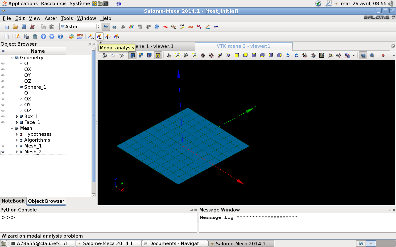
Figure 3.1-a: Location of the modal analysis wizard in Salomé-Méca.
The wizard simply asks the user to provide the mesh, to fill in the data on the materials, any boundary conditions. And finally the search criterion for specific modes (for example: the N first modes? or the modes on a given frequency band? or the modes around a target frequency?).
The wizard then automatically generates the Code_Aster command file, visible in the study tree, and that the user can open and edit (with the Eficas graphical interface or a text editor) if it is necessary, for example, to modify certain parameters or options.
Finally, the execution of the calculation automatically generates a message file (extension.mess) containing the details of all the calculations, as well as a result file (in MED format) containing the specific modes. You can open this file in the ParAvis module in order to visualize the deformations (paragraph 5.1).
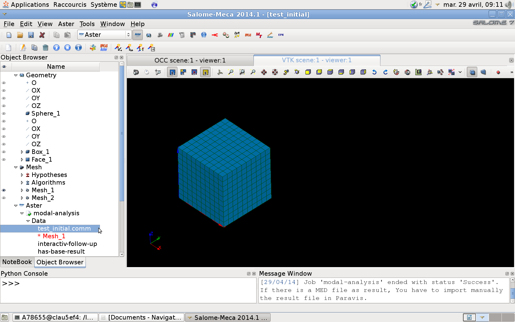
Figure 3.1-b: Command file generated by the wizard. |
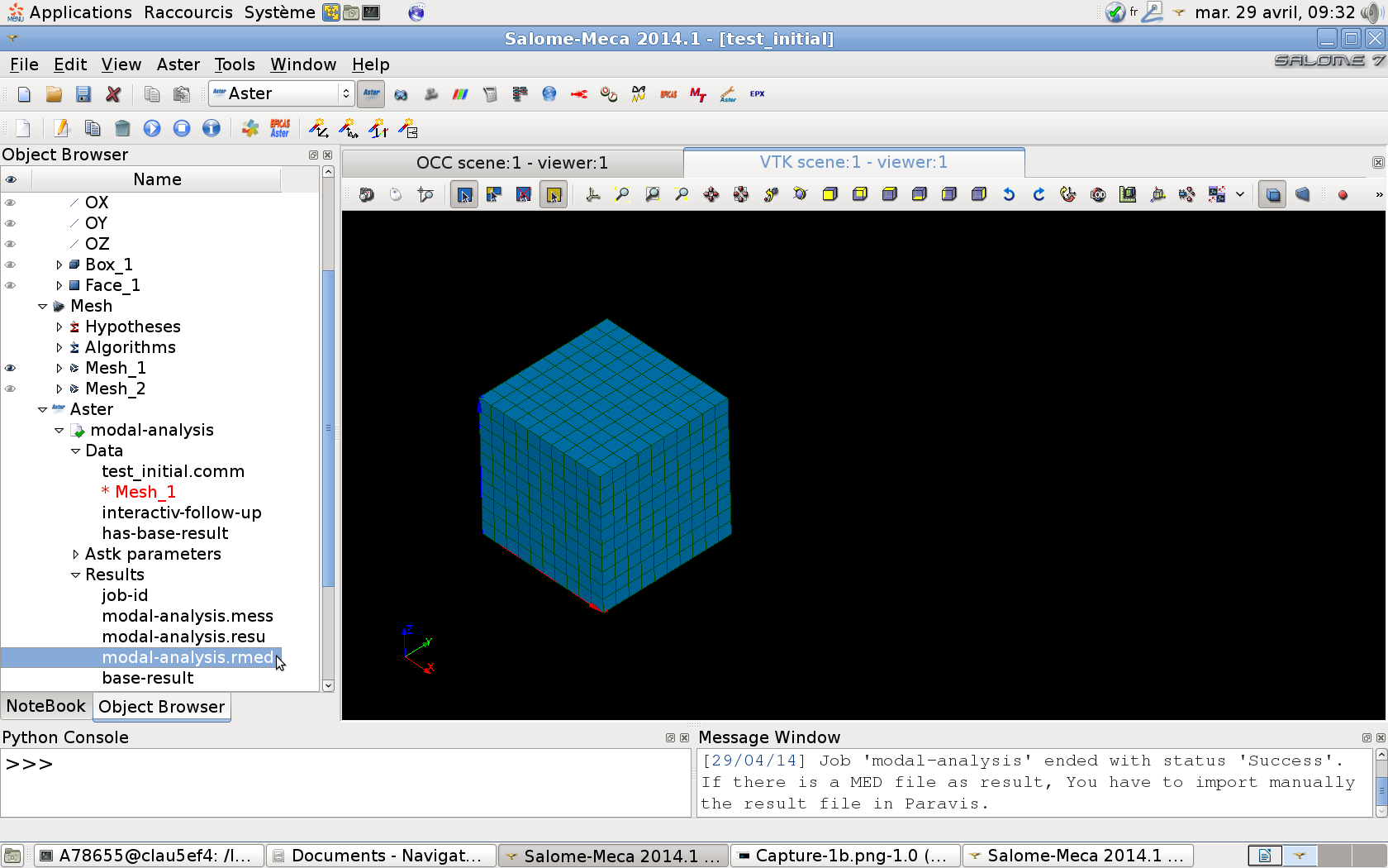
Figure 3.1-c: Result file generated by the wizard. |
3.2. More advanced features#
3.2.1. Code_Aster command chain#
From the input data, we proceed as follows:
calculation of assembled matrices (operator ASSEMBLAGE with the options” RIGI_MECA “and” MASS_MECA “; other options exist to calculate more specific matrices, for example geometric rigidity, damping, gyroscopy, etc.);
calculation of natural modes: operator CALC_MODES, with the keyword OPTION and the keyword factor CALC_FREQ used to specify the search criterion.
OPTION =” BANDE “or” PLUS_PETITE “or” CENTRE “or” TOUT “is to be preferred for its performance CPU if you are looking for a relatively large number of modes (up to 50 to 80; beyond that, we recommend dividing the search into several sub-bands, see paragraph 3.2.4.1), in particular with the search option on a given band ( OPTION =” BANDE “) for better robustness.
On the contrary, OPTION =” PROCHE “or” SEPARE “or” AJUSTE “, which is more expensive, should be used instead to calculate some modes with very good quality, for example if we want to refine initial estimates of eigenmodes (cf. paragraph 3.2.3).
At first, it is advisable to leave the default parameters of these operators, and to specify only the search criteria for the natural frequencies (by default, the first 10 modes).
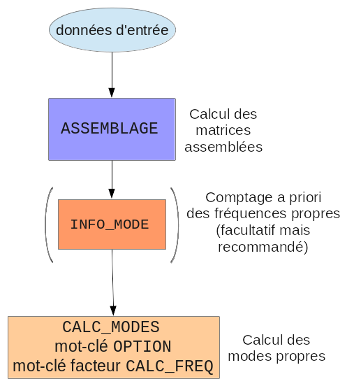
Figure 3.2-a : Calculation of modes using assembled matrices.
Example:
natural mode calculation on band \(\mathrm{[}\mathrm{20 };300\mathrm{]}\mathit{Hz}\):
ASSEMBLAGE (MODELE = model,
CHAM_MATER = ch_mat,
CARA_ELEM = cara_el,
CHARGE = c_limit,
NUME_DDL = CO (« numerota »), # creation of a numbering of
# DDL
MATR_ASSE =(
_F (MATRICE = CO (« matr_k »), OPTION = “RIGI_MECA”),
_F (MATRICE = CO (« matr_m »), OPTION = “MASS_MECA”),
)
)
modes = CALC_MODES (MATR_RIGI = matr_k,
MATR_MASS = matr_m,
OPTION = “BANDE”,
CALC_FREQ =_F (FREQ = (20., 300.))
)
3.2.2. Usefulness of an intermediate calculation of assembled matrices: some examples#
3.2.2.1. Prior counting of natural frequencies#
Before the actual calculation of the natural modes, it is strongly recommended to count the natural modes contained in one or more given frequency bands (in the standard case of real modes; if the modes to be calculated are complex, it will be a count around a point on the complex plane). This counting is much faster than the actual calculation of natural modes.
Knowing a priori the number of natural frequencies contained in the search band has a double utility in verifying and optimizing performances CPU of modal calculation:
verification: we can verify that the number of natural modes calculated by the modal solver is actually equal to the number of natural modes counted*a priori;
optimization CPU: if the number of natural frequencies counted on the search frequency band is too high (a threshold between 50 and 80 is commonly found), the user will be able to split his search band into several sub-bands, thanks to the CALC_MODES operator, with the operator with the option “BANDE” divided into sub-bands (see paragraph 3.2.4.1).
The natural modes are counted by the operator INFO_MODE. In a first approach, the user can simply fill in:
in the standard case of real modes: the matrices of the structure with the keywords MATR_ as well as its search band (s) with the keyword FREQ;
in the case of complex modes (structures with damping for example): you must specify TYPE_MODE =” COMPLEXE “and enter the search disk in the complex plane with RAYON_CONTOUR (and possibly CENTRE_CONTOUR) instead of FREQ.
3.2.2.2. Structures with hysteretic damping#
It is necessary to explicitly calculate the assembled total stiffness matrix including the hysteretic contribution (complex matrix).
The sequence of operators is as follows:
calculation of the assembled hysteretic stiffness matrices (calculated from the elastic stiffness matrix) and mass matrices (ASSEMBLAGE with the options” RIGI_MECA_HYST “and” MASS_MECA “respectively);
modal calculation with the hysteretic stiffness matrix (complex) and the mass matrix (CALC_MODES) as input.
Refer to the [U2.06.03] documentation for more information on taking hysteretic damping into account in*Code_Aster*.
3.2.2.3. Taking pre-constraints into account#
Taking into account pre-stresses (non-zero boundary conditions, static external loads, etc.) requires calculating the assembled mechanical and geometric stiffness matrices. They can then be combined to form the assembled total stiffness matrix which is the one used for the modal calculation.
The sequence of operators is as follows, in a relatively simple case of static external loading:
definition of external loading (operator AFFE_CHAR_MECA, with for example the FORCE_NODALE keyword),
calculation of the constraint field associated with this load (operator MECA_STATIQUE or STAT_NON_LINE or MACRO_ELAS_MULT to calculate the static response, then CREA_CHAMP with the keyword OPERATION =” EXTR “to retrieve the constraint field),
calculation of assembled matrices of mechanical stiffness, geometric rigidity associated with the stress field, and mass (ASSEMBLAGE),
combination of mechanical stiffness and geometric stiffness matrices to form the total stiffness matrix (COMB_MATR_ASSE),
modal calculation with the total stiffness matrix and the mass matrix as input (CALC_MODES).
Example:
Test case SDLL101 shows an example of calculating the modes of a beam subjected to static forces.
3.2.2.4. Taking into account gyroscopy (rotating machines)#
In addition to the other assembled matrices (stiffness, mass and possibly damping other than gyroscopic), the gyroscopic damping matrix must be calculated with the option “MECA_GYRO”. The operator CALC_MODE_ROTATION then makes it possible to calculate the natural modes of the structure for various speeds of rotation defined by the user under the keyword VITE_ROTA.
It is then possible to draw the Campbell diagram (evolution of natural frequencies as a function of the speed of rotation) of the rotating structure using the operator IMPR_DIAG_CAMPBELL.
Note:
The operator CALC_MODE_ROTATION is in reality a macro-command calling CALC_MODES: if necessary, the user can therefore perform the various elementary steps of CALC_MODE_ROTATION « by hand » but in a much less ergonomic manner*. Test case SDLL129 illustrates the approach in the case of a rotor with bearings whose characteristics depend on the speed of rotation.*
3.2.2.5. Use of modes for dynamic calculation on a modal basis#
Here too, you must have access to assembled matrices: their projection on a modal basis provides generalized matrices that can be used for dynamic calculation, with performances CPU much better than the direct use of assembled matrices. This model reduction method is described in the reference [R5.06.01] and usage documentation [U2.06.04].
3.2.3. Improving the quality of clean modes#
Attention is drawn to the fact that the quality of a modal calculation depends above all on the quality of the input data and the physical modeling. In particular, mention may be made of:
the choice of boundary conditions: are they representative of reality? Their influence is strong on the result of the calculation;
the fineness of the mesh: a mesh convergence study is necessary, as for any numerical study;
the choice of modeling: by structural elements (beam, shell,…) or in 3D? For example, for a slender structure, beam modeling will generally be better than 3D modeling even with good mesh fineness.
If the input data and the modeling are fixed, it is possible to improve the « computer » quality of the result thanks to the keyword AMELIORATION =” OUI “which automatically performs a chain of two modal calculations: the first which gives a first estimate of the natural modes (natural frequencies, modal deformations,…) with the search criterion requested by the user (for example with CALC_FREQ/OPTION =” BANDE “or” PLUS_PETITE “which use the subspace method), the second by the inverse power method (CALC_FREQ/OPTION =” PROCHE”) which refines the estimate of the previous calculation.
Rq 1: The first estimate is generally already good and satisfactory. For more complicated models, however, it is advisable to make this improvement.
Rq 2: this automatic functionality is limited to cases where the structure is represented by real symmetric matrices, and does not include multiple modes or multiple rigid body modes. For other cases, or if, for example, we only want to improve certain modes among all those calculated, we can of course do the calculations sequencing manually.
The sequence of commands is then as follows:
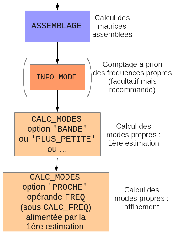
Figure 3.2-b : Improving the quality of clean modes (done manually) .
Example:
The first calculation of modes on the [0; 2000] Hz band with the command below:
mode1 = CALC_MODES (MATR_RIGI = k_asse,
MATR_MASS = mass,
OPTION = “BANDE”,
CALC_FREQ =_F (FREQ = (0., 2000.)),
)
gives the following results, visible in file MESSAGE:
LES FREQUENCES CALCULEES INF. AND SUP. SONT:
FREQ_INF: 4.65661E+01
FREQ_SUP: 1.60171E+03
CALCUL MODAL: METHODE OF ITERATION SIMULTANEE
METHODE OF SORENSEN
NUMERO FREQUENCE (HZ) NORME D’ERREUR
1 4.65661E+01 1.82405E-07
2 2.91827E+02 3.47786E-09
3 8.17182E+02 9.83625E-11
4 1.60171E+03 4.31692E-11
NORME from ERREUR MOYENNE: 0.46506E-07
VERIFICATION A POSTERIORI DES MODES
DANS THE INTERVALLE (4.64496E+01, 1.60571E+03)
THERE IS BIEN 4 FREQUENCE (S)
For example, it is possible to refine the first two natural modes, by launching the second calculation using the natural frequencies previously calculated:
mode2 = CALC_MODES (MATR_RIGI = k_asse,
MATR_MASS = mass,
OPTION = “PROCHE”,
CALC_FREQ =_F (FREQ = (46.6, 291.8)),
)
What gives
CALCUL MODAL: METHODE OF ITERATION INVERSE
INVERSE
NUMERO FREQUENCE (HZ) AMORTISSEMENT NB_ITER PRECISION NORME D’ERREUR
1 4.65661E+01 0.00000E+00 3 3.33067E-16 3.99228E-08
2 2.91827E+02 0.00000E+00 3 2.22045E-16 1.23003E-09
We can see that the error standard is slightly improved (admittedly slightly but this is a very simple case).
Note:
You can also automate the recovery of natural frequencies from the first estimate to feed the second calculation, using the Python language:
# retrieving the the list of estimated natural frequencies in the Python variable f_estimation:
f_estimate = mode1. LIST_VARI_ACCES () [“FREQ”]
mode2 = CALC_MODES (MATR_RIGI = k_asse,
MATR_MASS = mass,
OPTION = “PROCHE”,
CALC_FREQ =_F (FREQ = f_estimate),
)
3.2.4. Performance Optimization CPU#
3.2.4.1. Breakdown of the search frequency band#
If we are looking for a lot of specific modes (either because the search band is very broad, or because the modal density is high), the performance of the modal calculation will be better by dividing the global search band \(\left[{f}_{\mathit{min}};{f}_{\mathit{max}}\right]\) into several (\(n\)) sub-bands: \(\left[{f}_{\mathit{min}};{f}_{2}\right]\), \(\left[{f}_{2};{f}_{3}\right]\),…, \(\left[{f}_{n};{f}_{\mathit{max}}\right]\). This is done using the operator CALC_MODES with the option “BANDE” and by specifying the frequency division with the keyword FREQ =( fmin, f2,… , fn, fmax). To define the sub-bands, the user can rely on the a priori count of natural frequencies provided by the operator INFO_MODE, which can also operate by sub-bands.
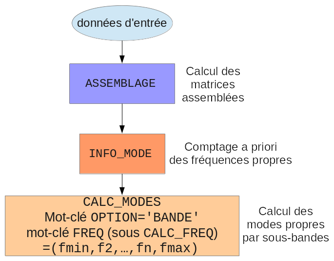
Figure 3.2-c : Calculation of natural modes by division into sub-bands.
Example:
identical to paragraph 3.2.1 by splitting the \(\mathrm{[}\mathrm{20 };300\mathrm{]}\mathit{Hz}\) band into three sub-bands:
ASSEMBLAGE (MODELE = model,
CHAM_MATER = ch_mat,
CARA_ELEM = cara_el,
CHARGE = c_limit,
NUME_DDL = CO (« numerota »), # creation of a numbering of
# DDL
MATR_ASSE =(
_F (MATRICE = CO (« matr_k »), OPTION = “RIGI_MECA”),
_F (MATRICE = CO (« matr_m »), OPTION = “MASS_MECA”),
)
);
nb_modes = INFO_MODE (MATR_RIGI = matr_k,
MATR_MASS = matr_m,
FREQ = (20.,300. ),
);
modes = CALC_MODES (MATR_RIGI = matr_k,
MATR_MASS = matr_m,
CALC_FREQ =_F (FREQ = (20., 100., 100., 200., 300.))
);
Notes:
There is a performance gain CPU even when sub-bands are processed sequentially (which is the case by default). The implementation of parallelism (see next paragraph) makes it possible to improve performance even more.
For optimal performance, it is advisable to have sub-bands that are as balanced as possible (i.e. with a relatively uniform number of modes per sub-band) .
3.2.4.2. Parallelism#
For modal calculation, parallelism can be implemented at two levels:
parallelization of the modal calculations carried out on each sub-band, in operators INFO_MODE and CALC_MODES with the option “BANDE” divided into several sub-bands;
parallelism at the level of the linear solver MUMPS, in the CALC_MODES operator when used with OPTION =” BANDE “or” PLUS_PETITE “or” CENTRE “or” TOUT “.
To implement parallelism, you need to:
have a version of*Code_Aster built with a parallel compiler (for example: Open MPI,…). On the centralized Aster4 server, parallel versions already exist: STAxx_impi;
select a parallel version of*Code_Aster in ASTK;
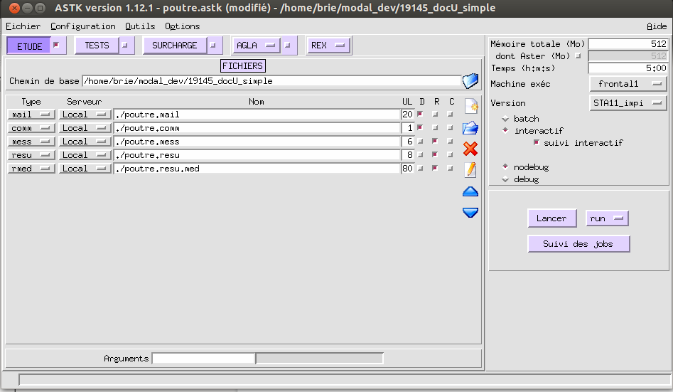
Figure 3.2-d : Selection in ASTK of a parallel version of Code_Aster (example on the centralized Aster4 server) .
specify in ASTK the number of processors and computing nodes to be exploited; you must use at least as many processors as there are non-empty frequency sub-bands, and it is recommended to use a number of processors that is multiple of the number of non-empty sub-bands (for example: if there are 5 non-empty sub-bands, use 10 or 15 or… processors);
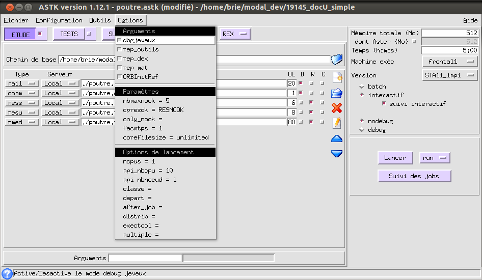
Figure 3.2-e : Declaration in ASTK of the number of processors and compute nodes to be exploited.
In the*Code_Aster command file:
to use the basic mode (parallelization of sub-bands only) with INFO_MODE or CALC_MODES with the “BANDE” option divided into several sub-bands, there is nothing to do: the keywords by default activate the parallelization of sub-bands;
to use the advanced mode (parallelization of the sub-bands for INFO_MODE and CALC_MODES with the “BANDE” option divided into several sub-bands, and the linear solver for all the modal operators): use the linear solver MUMPS (keyword factor SOLVEUR, keyword factor, operand METHODE =” MUMPS “; we also recommend setting the operands RENUM =” QAMD “and GESTION_MEMOIRE =” IN_CORE”).
Example:
identical to paragraph 3.2.4.1 by parallelizing both the calculations on the sub-bands and the linear solver:
modes = CALC_MODES (MATR_RIGI = matr_k,
MATR_MASS = matr_m,

CALC_FREQ =_F (FREQ = (20., 100., 100., 200., 300.)),
NIVEAU_PARALLELISME = “COMPLET”,
SOLVEUR =_F (METHODE = “MUMPS”,
RENUM = “QAMD”,
GESTION_MEMOIRE = “IN_CORE”),
);
Note:
For optimal performance, it is recommended to have sub-bands that are as balanced as possible (i.e.: with a relatively uniform number of modes per sub-band) .
The implementation of parallelism is presented in more detail in the generic documentation [U2.08.06] and the documentation for using INFO_MODE [U4.52.01] and CALC_MODES with the “BANDE” option divided into several sub-bands [U4.52.02].
3.2.4.3. Model reduction: calculation by substructuring#
When the numerical model has a large number of degrees of freedom or when the structure under study is an assembly of separately meshed components, methods for reducing the model by substructuring can be used, which are based on a geometric partitioning of the overall structure. On large models, these methods have better CPU performances than a direct calculation.
Dynamic substructuring
This method has a very general field of application. The [U2.07.05] documentation details its implementation.
Cyclic substructuring
This method has a much more restrictive field of application than the previous one: it makes it possible to treat only structures with cyclic repetitiveness (for example: bladed wheel,…). Test case SDLV301 provides an example of implementation.