5. Memory consumption RAM#
At each moment, the memory RAM used by****Code_Aster** can be the accumulation of three components.
Memory allocated directly by code sources. This is mainly the memory allocated by the software package JEVEUX [D6.02.01] to manage all F77 code data structures. This software package also allows these objects to be unloaded onto disk (Out-Of-Core functionality). Depending on the size of the problem, that of RAM and the programmer’s recommendations, JEVEUX performs more or less pronounced data exchanges between the disk and the RAM.
The**memory used by external software**requested by the*Aster calculation (MUMPS/PETSc, METIS/SCOTCH, HOMARD, MISS3D…). Most external software works in In-Core. That is to say, they do not directly manage possible memory overflows and that they outsource this task to the operating system. Others, like the linear solver MUMPS, are potentially OOC and they themselves explicitly manage the unloading of certain large objects onto disk (cf. keyword SOLVEUR/GESTION_MEMOIRE [U4.50.01]).
The**memory required by the system* (loading part of the executable, network layer in parallel…) and by the supervisor and the Python libraries.
When using a Code_Aster operator requiring the construction and resolution of linear systems (e.g. STAT_NON_LINE or CALC_MODES), memory limitations are often imposed by the linear solver (cf. [U4.50.01] [U2.08.03]). When it comes to internal solvers (LDLT, MULT_FRONT, GCPC), their RAM consumption is found in the JEVEUX displays. On the other hand, when using an external product (MUMPS or PETSC), you must then take into account your own consumption (which largely replace that of JEVEUX).
Resolution*via* MUMPS
**usol*
Calculation process
Linear system construction
Ku=F
Consumption RAM
Memory MUMPS
Memory JEVEUX
Figure 5-a: Diagram of evolution of consumption RAM during
of a standard calculation in linear mechanics.
5.1. Memory calibration of a calculation#
It is often interesting to calibrate an Aster calculation at the memory level RAM . This can, for example, make it possible to optimize its placement in a batch class (sequential or parallel) or simply avoid its sudden stop due to a memory defect. To do this, you can proceed as follows:
Step n° 1: identify in the calculation process the operator that seems the most dimensioning in terms of problem size (it is often the STAT/DYNA_NON_LINEou the CALC_MODES… dealing with the largest model).
Step 2: if this is not the case, set the block SOLVEURde to this operator with METHODE =” MUMPS “and GESTION_MEMOIRE =” EVAL “. At the end of the calibration, possibly remember to put the old settings back on.
Step 3: start the calculation as it is with modest memory and time parameters compared to the usual consumption of this type of calculation. Indeed, with this option, Code_Aster will just build the first linear operator system and send it to MUMPS for analysis. The latter will not perform its most expensive step (in time and especially in memory) of numerical factorization. Once this analysis is complete, the memory estimates for MUMPS (\({\mathit{MUE}}_{\mathit{IC}}\) and \({\mathit{MUE}}_{\mathit{OOC}}\)), together with that of JEVEUX (\({\mathit{JE}}_{\mathit{OOC}}\)), are plotted in the message file (cf. figure 5.1-a). Then the calculation stops at ERREUR FATALEafin to allow us to move on as quickly as possible to the next step.


===> Pour ce calcul, il faut donc une quantité de mémoire RAM au minimum de - 3500 Mo si GESTION_MEMOIRE=”IN_CORE”, - 500 Mo si GESTION_MEMOIRE=”OUT_OF_CORE”. En cas de doute, utilisez GESTION_MEMOIRE=”AUTO”. ************************************************************************** |
===> Pour ce calcul, il faut donc une quantité de mémoire RAM au minimum de - 3500 Mo si GESTION_MEMOIRE=”IN_CORE”, - 500 Mo si GESTION_MEMOIRE=”OUT_OF_CORE”. En cas de doute, utilisez GESTION_MEMOIRE=”AUTO”. ************************************************************************** |
Figure 5.1-a : Display in the message file in “ EVAL mode.
Step No. 4: exploitation of the memory estimates themselves.
To restart the calculation with the linear solver MUMPS, we have direct access to the « floor » values of the RAM memory that are essential for the calculation. There are two scenarios depending on the memory management mode of MUMPS chosen: In-Core (value \(\mathit{max}({\mathit{JE}}_{\mathit{OOC}},{\mathit{MUE}}_{\mathit{IC}})\) if GESTION_MEMOIRE =” IN_CORE “) or Out-Of-Core (value \(\mathit{max}({\mathit{JE}}_{\mathit{OOC}},{\mathit{MUE}}_{\mathit{OOC}})\) if GESTION_MEMOIRE =” OUT_OF_CORE”). Depending on the machine/batch classes you have, you must therefore restart the complete calculation by also possibly modifying this parameter of block SOLVEUR.
These estimates are established for a given computer and digital configuration: hardware platform, libraries, number of MPI processes, renumber, pre-treatments…
Step No. 4bis: on the other hand, if you want to restart the calculation by changing the linear solver or one of the numerical parameters, it is more difficult to deduce the adapted memory estimate. The combinatorics and the variability of the possibilities are too great. However, we can propose some empirical rules (in sequential mode). Roughly speaking, if instead of METHODE =” MUMPS “we choose” MULT_FRONT “the estimated memory should remain legal (with RENUM =” METIS” the default value). With “LDLT”, this figure must be significantly increased. With “PETSC”/”GCPC” + “LDLT_SP”, it can arguably be reduced to \(\mathit{max}({\mathit{JE}}_{\mathit{OOC}},{\mathit{MUE}}_{\text{IC/OOC}}\mathrm{/}2)\). With “PETSC”/”GCPC” + “LDLT_INC” it can probably be reduced to a factor of 1 times \({\mathit{JE}}_{\mathit{OOC}}\) depending on the level of filling of the preconditioner (keyword NIVE_REMPLISAGE cf. [R6.01.02]).
Step 5: restart the complete calculation by possibly modifying the settings of block SOLVEUR and by setting Astk with the value deduced in step 4 (« Total Memory (MB) » menu in Figure 5.2-b).
Note:
This memory calibration procedure for a study is only available since the restoration of the keyword SOLVEUR/GESTION_MEMOIRE (from version v11.2 of Code_Aster). For older versions, if the calculation has already been started (and if you have a usable message file), you can, at a minimum, carefully use as an optimal estimate of the required memory, the largest value on all the processors of the Vmpeak*of the last operator. Otherwise, proceed as mentioned in previous versions of this document:*
**Step 1: as above.*
**Step 2: set up the block* SOLVEURavec * METHODE =” MUMPS “,” OUT_OF_CORE “=” OUI “ and * and INFO =2.
**Step 3: start the calculation while limiting time consumption (for example, with few steps or few searches for natural modes) .*
**Step 4: depending on the memory management mode of MUMPS required (IC or OOC), take the maximum of the estimate MUMPS and the consumption* JEVEUX.
5.2. Memory consumption JEVEUX#
Elements to quantify the memory consumption of JEVEUX **** are plotted at the end of each Aster operator (cf. figure 5.2-a). Broadly speaking, they can be explained in the following way:
:math:`{mathit{JE}}_{mathit{OOC}}` provides the**minimum size**(“Minimum”)* you need JEVEUXpour to work up to this operator. It will then be completely Out-Of-Core (OOC). Below this value, the calculation is not possible (in the selected configuration).
\({\mathit{JE}}_{\mathit{IC}}\) provides a lower bound (“Optimum”), up to this operator, of the JEVEUX memory required to function completely in In-Core (IC): \({\mathit{JE}}_{\mathit{IC}}^{\text{'}}\). With at least this memory value RAM set in Astk (see \({\mathit{MEM}}_{\mathit{ASTK}}\)), the calculation will take place in an optimal manner: there is no risk of crashes due to a lack of memory and accesses to purely Aster data structures are not slowed down much by disk-loading.
These two figures are necessarily less than the total memory value RAM devoted to the calculation (set in Astk), noted \({\mathit{MEM}}_{\mathit{ASTK}}\).

# Memory Statistics (MB): 15521.78/ 8920.78/ 8920.14/ 1603.77/ 248.27 (VMPeak/VMSize/Optimum/Minimum)
Figure 5.2-a: Overall statistics at the end of each order

(extracted from a.mess).
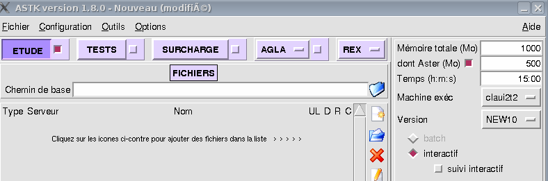
Figure 5.2-b: Parameterization of memory RAM in Astk.
Note:
If there was no global release mechanism (see paragraph below), \({\mathit{JE}}_{\mathit{IC}}\) truly represents the memory JEVEUX required to function in IC. Otherwise, this last estimate should be close to the sum [11] _ \({\mathit{JE}}_{\mathit{IC}}^{\text{'}}\mathrm{=}{\mathit{JE}}_{\mathit{IC}}+\mathrm{.}\) « the average gain from each release. » It is therefore useless (if you do not use an external product) to set up the calculation with a value much greater than \({\mathit{JE}}_{\mathit{IC}}^{\text{'}}\).
When configuring the calculation, a compromise must therefore be established between its speed and its memory consumption. By prioritizing the memory consumption of all the commands, it is possible to identify which one sizes the calculation. With a fixed calculation configuration (number of processors), the larger the memory space reserved for JEVEUX, the more In-Core (IC) the calculation will be and therefore the faster it will be. Depending on the contingencies of batch queues, you can also split your calculation into different POURSUITE in order to mix and thus optimize the « computation time/memory » settings.
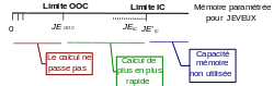
Figure 5.2-c :Meaning of displays linked to JEVEUX in the message file.
During the calculation, JEVEUXpeut unload a large portion of the RAM objects onto disk. This mechanism is either:
Automatic (there is no longer enough space RAM to create an object or bring it back),
Managed by the programmer (e.g. call to this release mechanism just before handing over to MUMPS).
The statistics concerning this mechanism are summarized at the end of the message file (see §5.2-d) for all orders. Obviously, the more this mechanism intervenes (and on large volumes of memory freed), the more the calculation is slowed down (system time and elapsed which increase and time CPU stable). This phenomenon may be accentuated in parallel mode (simultaneous memory containment) depending on the distribution of processors on the computing nodes and according to the characteristics of the machine.
STATISTIQUES CONCERNANT L” ALLOCATION DYNAMIQUE :
TAILLE CUMULEE MAXIMUM: 1604 MB.
TAILLE CUMULEE LIBEREE: 52117 MB.
NOMBRE TOTAL from ALLOCATIONS: 1088126

NOMBRE TOTAL FROM LIBERATIONS: 1088126
APPELS TO MECANISME FROM LIBERATION: 1
TAILLE MEMOIRE CUMULEE RECUPEREE: 1226 MB.
VOLUME DES LECTURES: 0 MB.
VOLUME DES ECRITURES: 1352 MB.
MEMOIRE JEVEUX MINIMALE REQUISE POUR L’EXECUTION: 248.27 MB
IMPOSE OF NOMBREUX ACCES DISQUE
RALENTIT THE VITESSE FROM EXECUTION
MEMOIRE JEVEUX OPTIMALE REQUISE POUR L’EXECUTION: 1603.77 MB
LIMITE LES ACCES DISQUE
AMELIORE THE VITESSE FROM EXECUTION
Figure 5.2-D: Statistics of the JEVEUX release mechanism (.mess).
These statistics also summarize the estimates \({\mathit{JE}}_{\mathit{IC}}\) and \({\mathit{JE}}_{\mathit{OOC}}\) detailed above.
Note:
Any additional costs in terms of these unloading times are traced at the end of the operators concerned (cf. §4.1.1). In the case of a lack of RAM, we can diagnose this one via the “VMPeak” parameter (cf. §5.4) .
5.3. External product memory consumption (MUMPS)#
For now, the only external product whose memory consumption RAM is really sizeable is the product MUMPS. You can track your consumption (In-Core and Out-Of-Core) in two ways:
By**a very fast and inexpensive pre-calculation**in memory*via mode GESTION_MEMOIRE =” EVAL “(see §5.1). But these are only estimates (values \({\mathit{ME}}_{\mathit{IC}}\) and \({\mathit{ME}}_{\mathit{OOC}}\) in Figure 5.1-a). They can therefore be a bit pessimistic (especially in Out-Of-Core and/or in parallel). In parallel mode, we only draw the estimates of the most demanding MPI process.
By**the standard calculation* (limited if possible to a few steps of time or to a few specific modes) by adding the keyword INFO =2 in the supposed most expensive command. In the message file (cf. 5.3-a), we then summarize not only the previous memory estimates \({\mathit{ME}}_{\mathit{IC}}\) and \({\mathit{ME}}_{\mathit{OOC}}\) (columns” ESTIM IN- CORE “and” ESTIM OUT -OF- CORE “), but also the actual consumption of the mode chosen \({\mathit{MR}}_{\text{IC/OOC}}\) (here in mode OOC because display” RESOL OUT -OF- CORE “). For example, in Figure 5.3-a, it should read: « MUMPS estimates that it needs at least \({\mathit{ME}}_{\mathit{OOC}}\mathrm{=}\mathrm{478Mo}\) per processor to function in OOC. To switch to IC (faster calculation), he estimates that he needs at least \({\mathit{ME}}_{\mathit{IC}}\mathrm{=}\mathrm{964Mo}\); in practice, he consumed exactly \({\mathit{MR}}_{\mathit{OOC}}\mathrm{=}\mathrm{478Mo}\) in OOC (the estimate is therefore perfect: \({\mathit{ME}}_{\mathit{OOC}}\mathrm{=}{\mathit{MR}}_{\mathit{OOC}}\)!).
In parallel mode, we summarize the numbers by process MPI, as well as their minima, maxima, and averages. It is an expertise-based display that is more detailed than the GESTION_MEMOIRE =” EVAL “mode display. In addition to this RAM consumption information, it also summarizes elements related to the type of problem, its numerical difficulty (errors) and its parallel distribution (load balance).
**********************************************************************************

< **MONITORING DMUMPS 4.8.4** >

TAILLE FROM SYSTEME 210131

**RANG** **** NBRE MAILLES **** **NBRE TERMES K** **LU FACTEURS**

NO. 0:5575 685783 45091154

N 1:8310 1067329 51704129

N 2:11207 1383976 53788943

...

N 7:8273 1039085 4560659

-----------------------------

TOTAL: 67200 8377971 256459966

**MEMOIRE RAM ESTIMEE AND REQUISEPAR MUMPS IN MO** (FAC_NUM + RESOL)

*MROOC*
**MASTER RANK: ESTIM IN-CORE | ESTIM OUT-OF-CORE | RESOLVED. OUT-OF-CORE**

*MEIC*

*MEOOC*
NO. 0:869 478 478

N 1:816 439 439

N 2:866 437 437

...

N 7:754 339 339

-----------------------------------------------------------------------------

**MOYENNE**: 5.92D+02 3.50D+02 3.50D+02

-----------------------------------------------------------------------------

**MINIMUM**: 7.54D+02 3.39D+02 3.39D+02

-----------------------------------------------------------------------------

**MAXIMUM**: 9.64D+02 4.78D+02 **4.78D+02**

-----------------------------------------------------------------------------

*************************************************************************************
Figure 5.3-a: Memory consumption per processor (estimated and realized) of the external product MUMPS (displayed in the .mess if INFO =2).
Notes:
Depending on the type of calculation (sequential, parallel, centralized or distributed), the number of processors, the mode of use of JEVEUX (keyword SOLVEUR/MATR_DISTRIBUEE) and the memory manager MUMPS (keyword SOLVEUR/GESTION_MEMOIRE), the memory hierarchy can however be upset. In distributed parallel mode, the memory peak JEVEUX will decrease with the number of processors as soon as MATR_DISTRIBUE is activated. This will also be the case for MUMPS , regardless of the parallelism mode (especially in IC). Moreover, the transition of MUMPS from IC mode to OOC mode will also drastically drop its memory peak.
The display in INFO =2 of the RAM of MUMPS consumptions by processor provides information on possible memory load imbalances. We can try to limit them by modifying the product scheduling heuristic: parameters SOLVEUR/PRETRAITEMENTS and RENUM or the number of processors.
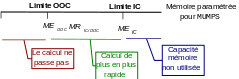
Figure 5.3-b: Meaning of displays linked to MUMPS in the message file.
5.4. System consumption#
The only system consumption mentioned in the message file concerns the overall memory of the job at this moment of the calculation (VMsize) and its peak from the start (VMpeak). It is plotted at the end of each order (cf. figures \({\mathit{SYS}}_{1}\mathrm{/}{\mathit{SYS}}_{2}\) figure 5.2a). The VMpeak is summarized at the end of the message file (cf. figure 5.4a).

MAXIMUM of MEMOIRE UTILISEE PAR LE PROCESSUS: 15107.89 MB
COMPREND THE MEMOIRE CONSOMMEE PAR JEVEUX,
THE SUPERVISEUR PYTHON, LES LIBRAIRIES EXTERNES
Figure 5.4-a: Final VMpeak of the Unix process.
In broad strokes VMPeak provides information about the peak in memory size caused by all the active executables of the Aster job. Care must be taken to ensure that this figure remains lower than the physical memory available to the job. Otherwise, the system will, up to a certain point, « swap » and this will slow down the calculation. At the level of the JEVEUX software package, this will result in more unloads (see §4.1.2 and §5.2) and, at the level of external products, in a growing ELAPS/USER gap (traced at the end of the order see §4.1.1).
Notes if SOLVEUR =” MUMPS “:
Since the rendering of the SOLVEUR/GESTION_MEMOIRE keyword (starting with Code_Aster version v11.2), the solver is allowed to « spread out » in memory, in addition to the JEVEUX /Python/libraries allocations, until it occupies the maximum size allocated. This allows the product to be faster and less picky about its memory needs in terms of pivoting. On the other hand, as a consequence of this strategy for optimum occupancy of memory resources, the VMpeak displayed in the message file becomes dependent on the memory allocated to the calculation (MEMASTKou terminal of the batch class). It cannot therefore be used, as before, to calibrate the minimum memory consumption of the study. To do this, you must instead apply the strategy detailed in §5.1