1. Calculation of the reinforcement of beams and columns#

1.1. Notations and principles of balance#

The internal forces of 1D structural elements (beams/columns) are expressed in the element’s local coordinate system, which will be defined here in a manner consistent with the [U4.81.82] documentation concerning the instructions for using the CALC_FERRAILLAGE command.

Thus, the X axis coincides with the supporting axis of the element, while the Y and Z axes are in the plane of the right section and parallel to its sides in accordance with the figure below.

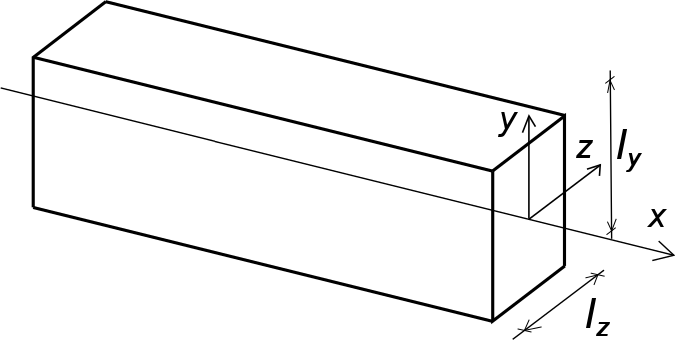
Figure 1. Definition of the axes of a linear element such as a beam/post

By using a rectangular cross-section beam, the code_aster command file defines the two sides of the rectangle \({l}_{y}\) and \({l}_{z}\) in the code_aster command file, making it possible to define the two main axes of inertia of the section, namely the axes \(y\) and \(z\).

The efforts expressed in the local coordinate system of the element are therefore:

\(N\): normal effort
\({V}_{y},{V}_{z}\): shear forces
\({M}_{y},{M}_{z}\): moments of bending
\({M}_{x}\): torsional moment

It should be noted that the moments are expressed in relation to the center of gravity of the unarmed section (center of the geometric section). In addition, it will be said that the section is subject to a:

simple flexuration if only a bending moment (\({M}_{y}\) or \({M}_{z}\)) stresses the section.
compound flexuration if a bending moment (\({M}_{y}\) or \({M}_{z}\)) and a normal force \(N\) act on the section.
compound deflected flex if the section is simultaneously subjected to both \(({M}_{y},{M}_{z})\) bending moments as well as to a normal force \(N.\)
compression or pure tract if only \(N\) acts on the section.

The typical reinforcement field of a beam/column is defined as follows, at the level of the cross section of the element:

4 beds of longitudinal reinforcement: \({A}_{\text{sy,sup}}\), \({A}_{\text{sy,inf}}\),,, \({A}_{\text{sz,sup}}\) and \({A}_{\text{sz,inf}}\) usually expressed in \({\mathit{cm}}^{2}\)

These sections are carried by the two main inertia axes Y and Z of the section.

a density/ratio of transverse reinforcement: \({A}_{\text{sv}}/s\) usually expressed as \({\mathit{cm}}^{2}/m\)

For this reason, the reinforcement is calculated in two stages:

calculation of the longitudinal reinforcement: composite and/or deviated flexural balance, with respect to the axial compression forces N, and the two moments of bending along the two inertia axes of the girder, namely My and Mz.
calculation of transverse reinforcement: balance at shear shear forces Vy and Vz, and at torsional moment Mx. It should then be noted, in accordance with the following explanations, that these forces may in some cases induce additional traction forces along the supporting axis X of the element, thus leading to an excess of longitudinal reinforcement.

These equilibrium calculations are therefore based on criteria related to the design limit state used, namely:

ELU: the criterion is that the ultimate deformations of compressed concrete and reinforcing steel have not been exceeded.
ELS Characteristic: the criterion is that the limit compressive stress of concrete under compression and the limit stress of flexural steel have not been exceeded.
ELS Quasi-Permanent: the criterion is that the maximum crack opening has not been exceeded.

1.2. Sizing at ELU#

1.2.1. Calculation of longitudinal reinforcement in simple or compound bending#

1.2.1.1. Definition of calculation hypotheses#

At ELUs, the principles for verifying the cross section and for the calculation of composite flexural reinforcement with respect to loads:math: `N, {M} _ {text {y|z}} `, are based on the following three hypotheses:

Straight cross sections remain flat after deformation (Euler-Bernoulli). Therefore, this implies that the deformation diagram governing the cross section at equilibrium in composite bending is linear as follows:
A limit threshold is imposed for deformations:

deformation of compressed concrete limited to \({\epsilon }_{\mathit{cu}2}\) (Pivot B), in the case of a partially stretched/compressed section

deformation of compressed concrete limited to \({\epsilon }_{c2}\) (Pivot C), in the case of a fully compressed section

The stress-strain diagrams for steel and concrete are as given below:

For compressed concrete:

Figure 2. Law of behavior of concrete under compression at ELU

For this reason, the following parameters are defined:

\({f}_{\mathit{ck}}\): characteristic value of compressive strength of concrete, which in practice is defined according to the concrete class at the level of Eurocode 2.
\({f}_{\mathit{cd}}\): value of the compressive strength of concrete used for the calculation in ELU, namely \({f}_{\mathit{cd}}=\frac{{\alpha }_{\mathit{cc}}{f}_{\mathit{ck}}}{{\gamma }_{c}}\), with \({\alpha }_{\mathit{cc}}=1\) for EC2 and \({\gamma }_{c}\) (safety coefficient) which depends on the type of ELU considered (1.5 in a permanent situation and 1.2 in an accidental situation).
\({\epsilon }_{c2}\): deformation reached for maximum stress. It is worth (formula in MPa):

\({\epsilon }_{c2}(\text{‰})=2+0.085{({f}_{\mathit{ck}}-50)}^{0.53}\) if \({f}_{\mathit{ck}}>50\mathit{MPa}\)

\({\epsilon }_{\mathit{cu}2}\): ultimate deformation of the concrete at break. It is worth (formula in MPa):

\({\epsilon }_{\mathit{cu}2}(\text{‰})=2.6+35{[(90-{f}_{\mathit{ck}})/100]}^{4}\) if \({f}_{\mathit{ck}}>50\mathit{MPa}\)

\(n\): parameter for the definition of the parabolic branch of the law of behavior, and which is equal (formula in MPa):

\(n=1.4+23.4{[(90-{f}_{\mathit{ck}})/100]}^{4}\) if \({f}_{\mathit{ck}}>50\mathit{MPa}\)

Thus, for deformation values for concrete \({\epsilon }_{c}\le {\epsilon }_{c2}\), the stress in the concrete is then calculated by the following formula:

\({\sigma }_{c}={f}_{\mathit{cd}}(1-{(1-{\epsilon }_{c}/{\epsilon }_{c2})}^{n})\)

It is also possible to carry out the calculation with the hypothesis of a « simplified rectangular diagram »: the stress of the concrete is then considered to be constant and equal to \(\eta {f}_{\mathit{cd}}\) over a height equal to \(\lambda x\) (fraction « \(\lambda\) » of the compressed zone). This simplification is suggested and accepted by Eurocode 2 (as long as the neutral axis remains within the section), since the error thus generated on the \({F}_{c}\) resultant of compression forces in concrete remains minimal.

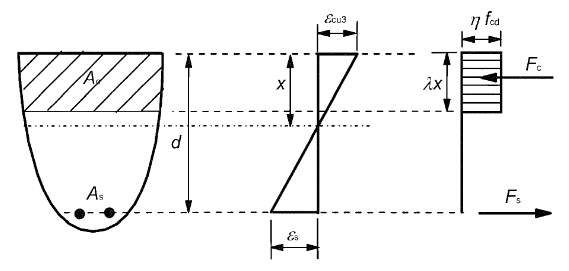
Figure 3. Simplified rectangular stress-strain diagram for concrete.

The values of \(\lambda =0.8\) and \(\eta =1\) should be used for common concrete (\({f}_{\mathit{ck}}⩽50\mathit{MPa}\)). For values \(50\mathit{MPa}<{f}_{\mathit{ck}}\le 90\mathit{MPa}\) we have:

\(\lambda =0.8-({f}_{\mathit{ck}}-50)/400\)

\(\eta =1-({f}_{\mathit{ck}}-50)/200\)

For reinforcing steel:

The behavior of steel recommended by Eurocode 2 in terms of stress-deformation is of the bilinear type. It is also possible to adopt perfect plastic behavior (horizontal level diagram in the following figure); the current version of the CALC_FERRAILLAGEde code_aster operator allows you to choose between these two types of diagrams using the TYPE_DIAGRAMME keyword.

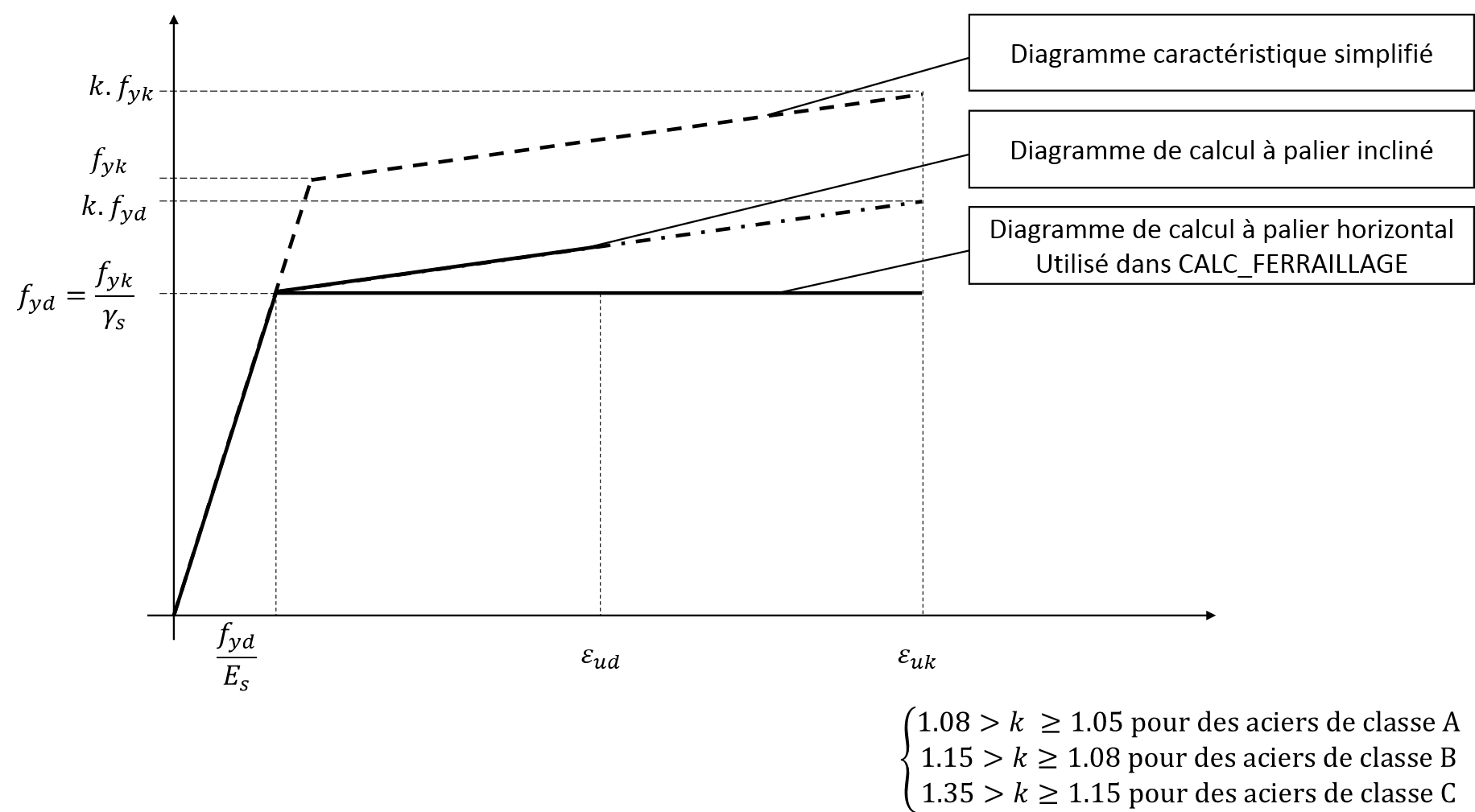
Figure 4. Stress-strain graph for flexure steel.

In the diagram presented above, the following parameters are identified:

The limiting stress of elastic behavior \({f}_{\mathit{yk}}\) which depends on the type of steel used
The limiting stress of the elastic behavior used for the calculation, namely \({f}_{\mathit{yd}}=\frac{{f}_{\mathit{yk}}}{{\gamma }_{s}}\), where \({\gamma }_{s}\) is a safety factor.
The ultimate deformation at break \({\epsilon }_{\mathit{uk}}\), which depends on the steel class used:

Class B: \({\epsilon }_{\mathit{uk}}=5\text{\%}\)

Class C: \({\epsilon }_{\mathit{uk}}=7.5\text{\%}\)

The ultimate deformation at break used for the calculation, namely \({\epsilon }_{\mathit{ud}}=0.9{\epsilon }_{\mathit{uk}}\).
Parameter \(k\) in the figure above (only required when using an inclined bearing) is defined by \(k={({f}_{t}/{f}_{y})}_{k}\), with \({f}_{t}\) the ultimate breaking stress. The value of this parameter also varies according to the steel class (A, B or C) as indicated in the preceding figure.
The \({E}_{s}\) Young’s modulus of steel (mean value and not characteristic). Among other things, the limit of elastic deformation behavior is then defined, namely \({{\epsilon }_{\mathit{yd}}=f}_{\mathit{yd}}/{E}_{s}\).

Apart from Young’s modulus, it is the design values (index « d ») that are used in dimensioning or verification calculations.

1.2.1.2. Balance principle and calculation of steel sections#

The hypotheses introduced in §1.2.1.1 are used to draw the diagram in the following Figure and are at the origin of the « rule of three pivots » used to size or verify a reinforced concrete section.

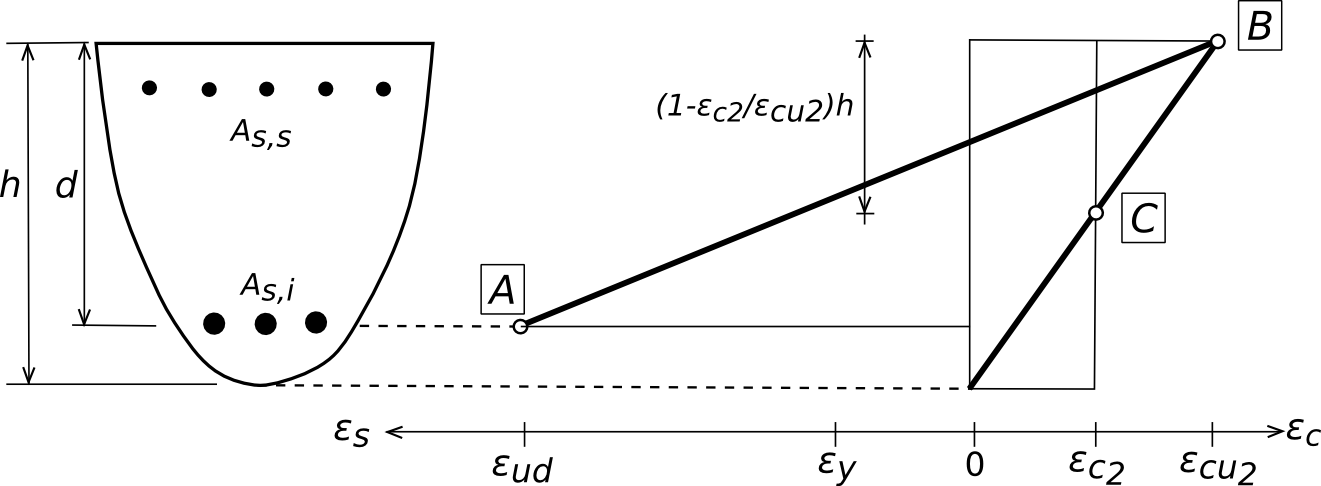
Figure 5. Principle of dimensioning in composite flexure at ELU

In the figure above, we can distinguish:

A typical concrete section with a lower reinforcement \({A}_{s,i}\) and an upper \({A}_{s,s}\) reinforcement, with a height equal to \(h\) and a useful height \(d\), which represents the lever arm of the center of gravity of the lower reinforcements in relation to the upper fiber of the section* (in the case of a negative moment of bending, this is then the lever arm of the center of gravity of the upper reinforcements in relation to the lower fiber of the section) . In practice, it can be estimated that :math:`d=h-{c}_{mathit{inf}}`, such as cinf represents the embedding (within a half-diameter of the reinforcement) of the lower reinforcements, that is to say the distance of the center of gravity of the lower reinforcements in relation to the lower fiber of the section (in the context of a negative bending moment, * we then consider d = h-csup) .
The drawing of the limit deformation diagrams, in the form of lines in the form of lines for the Euler-Bernoulli hypothesis, through the 3 pivots A, B and C.

The design at ELU consists in placing oneself under failure conditions corresponding to the achievement of a limit deformation relating to either steel or concrete, so that the deformation diagram passes through one of the three points A, B, C schematised in the previous figure:

Pivot A corresponds to the failure of the lower steel* (in the context of a negative bending moment, it is then the upper steel) *, i.e. when the tensile steel reaches the deformation limit \({\epsilon }_{\mathit{ud}}\)
Pivot B corresponds to the rupture of the upper fiber concrete* (in the context of a negative bending moment, it is then the lower fiber concrete) *, i.e. when the most compressed concrete reaches the deformation limit \({\epsilon }_{\mathit{cu}2}\)
Pivot C corresponds to the achievement of the maximum strength \({f}_{\mathit{cd}}\) of concrete (in accordance with the law of behavior represented in FIG. 3), i.e. for a deformation equal to \({\epsilon }_{c2}\). This pivot is used for the study of fully compressed cases; its position in relation to the height of the section is obtained from the intersection of the diagram relating to the limit of the partially compressed case (neutral axis positioned at the level of the lower fiber* (in the case of a negative bending moment, it is then the upper fiber) * from the straight section (BC)) and from the case of pure compression (\({\epsilon }_{c2}\) over the entire height of the section). For the latter case (pure compression), Eurocode 2 thus prefers to limit concrete deformations to \({\epsilon }_{c2}\) rather than \({\epsilon }_{\mathit{cu}2}\).

The points A, B, C are called « pivots » since it is possible to scan all the possible fracture configurations of the section by pivoting around one of them.

In fact, based on the definition of the three pivots and the position of the neutral axis of the deformation diagram, it is possible to define break « domains », as represented in the following figure:

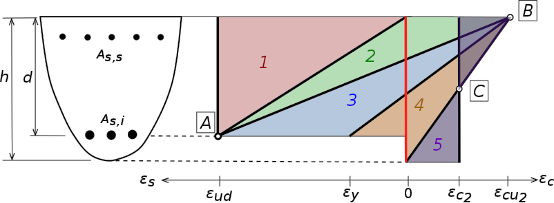
Figure 6. Domains of function/balance in flexure composed at ELU.

Domain 1: The deformation diagram goes through PIVOT A, but the neutral axis is outside the section and above the upper fiber, such that the entire section is under tension.

Domain 2: The deformation diagram always goes through PIVOT A, but the neutral axis is now inside the section. The section is thus partially compressed, such that the break is in line with the tensile steel.

Domain 3: the deformation diagram now goes through PIVOT B, and the neutral axis is inside the section. The section is therefore still partially compressed, with a break at the right of the upper fiber of the concrete.

Domain 4: it is a continuation of the hypotheses of the previous field, but the deformation of lower steel becomes less than the limit of elastic-plastic behavior, namely \({{\epsilon }_{\mathit{yd}}=f}_{\mathit{yd}}/{E}_{s}\). Tensile steel falls into the elastic domain and therefore no longer works optimally in terms of strength.

Domain 5: the neutral axis is again outside the section, but below the lower fiber. The section is now fully compressed, such that the deformation diagram goes through PIVOT C.

Depending on the torsor of forces applied, the algorithm will then determine the optimum operating range for the balance; the upper and lower reinforcement sections are then calculated from the equations for the balance of forces and moments, as explained below.

In accordance with the preceding notations, when \(M>0\), the moment and the reduced moment are calculated at the center of gravity of the lower reinforcements, such as (the normal force \(N\) being positive under compression):

\({M}_{\text{inf}}=M+N\mathrm{.}\left(\frac{h}{2}-{c}_{\text{inf}}\right)\)

\({\mathrm{\mu }}_{\text{inf}}=\frac{{M}_{\text{inf}}}{b\mathrm{.}d\mathrm{²}\mathrm{.}\mathrm{\eta }\mathrm{.}{f}_{\mathit{cd}}}\)

In the same way when \(M<0\), the moment and the reduced moment are calculated at the center of gravity of the upper reinforcements, such as:

\({M}_{\text{sup}}=-M+N\mathrm{.}\left(\frac{h}{2}-{c}_{\text{sup}}\right)\)

\({\mathrm{\mu }}_{\text{sup}}=\frac{{M}_{\text{sup}}}{b\mathrm{.}d\mathrm{²}\mathrm{.}\mathrm{\eta }\mathrm{.}{f}_{\mathit{cd}}}\)

Next, we consider the case of positive bending (the results of the M<0 case are then obtained symmetrically).

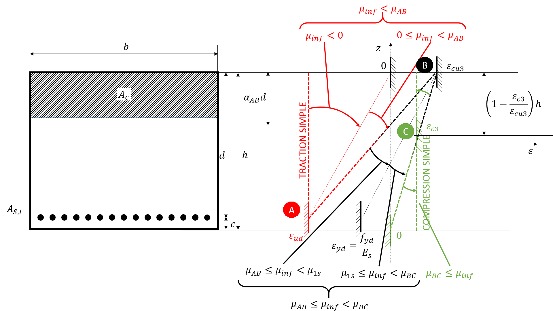
Figure 7. Principle of the rule of three pivots for a rectangular section (hxb)

Considering a partially compressed section (that is to say that the neutral axis \(x=\mathrm{\alpha }\times d\) of the deformation diagram is inside the section; in concrete terms, this corresponds to the domain \(0⩽\mathrm{\alpha }⩽1\)), in the absence of compression steel (that is to say that \({A}_{s,s}=0\)) and with the notations in FIG. 3, the resistant moment of the section expressed at the center of gravity of the tensile steel is provided exclusively by compressed concrete, and is expressed as follows:

\({M}_{\text{c}}=\mathrm{\alpha }\mathrm{\lambda }\mathit{db}\times \mathrm{\eta }{f}_{\mathit{cd}}\times (d-\mathrm{\alpha }\mathrm{\lambda }d/2)=({\mathit{bd}}^{2}\mathrm{\eta }{f}_{\mathit{cd}})\times \mathrm{\lambda }\mathrm{\alpha }(1-\mathrm{0,5}\mathrm{\lambda }\mathrm{\alpha })\)

Or even, at a reduced moment:

\({\mathrm{\mu }}_{\text{c}}=\frac{{M}_{c}}{{\mathit{bd}}^{2}\mathrm{\eta }{f}_{\mathit{cd}}}=\mathrm{\lambda }\mathrm{\alpha }(1-\mathrm{0,5}\mathrm{\lambda }\mathrm{\alpha })\)

The balance of moments then leads to having: \({\mathrm{\mu }}_{\text{c}}=\mathrm{\lambda }\mathrm{\alpha }(1-\mathrm{0,5}\mathrm{\lambda }\mathrm{\alpha })={\mathrm{\mu }}_{\text{inf}}\)

Solving this 2nd degree equation then makes it possible to determine the value of the depth coefficient of the neutral axis α. Depending on the value of this coefficient, we find ourselves in one of the 5 balance domains stipulated previously in the documentation, namely:

Domain 1: \(\mathrm{\alpha }⩽0\) and \(\mathrm{\mu }⩽0\)
Domain 2: \(0⩽\mathrm{\alpha }⩽{\mathrm{\alpha }}_{\mathit{AB}}\) and \(0⩽\mathrm{\mu }⩽{\mathrm{\mu }}_{\mathit{AB}}\),

such as \({\mathrm{\alpha }}_{\mathit{AB}}=\frac{1}{1+{\mathrm{\epsilon }}_{\mathit{ud}}/{\mathrm{\epsilon }}_{\mathit{cu}3}}\) and \({\mathrm{\mu }}_{\mathit{AB}}=\mathrm{\lambda }{\mathrm{\alpha }}_{\mathit{AB}}(1-\mathrm{0,5}\mathrm{\lambda }{\mathrm{\alpha }}_{\mathit{AB}})\)

Domain 3: \({\mathrm{\alpha }}_{\mathit{AB}}⩽\mathrm{\alpha }⩽{\mathrm{\alpha }}_{R}\) and \({\mathrm{\mu }}_{\mathit{AB}}⩽\mathrm{\mu }⩽{\mathrm{\mu }}_{R}\),

such as \({\mathrm{\alpha }}_{R}=\frac{1}{1+{\mathrm{\epsilon }}_{\mathit{yd}}/{\mathrm{\epsilon }}_{\mathit{cu}3}}\) and \({\mathrm{\mu }}_{R}=\mathrm{\lambda }{\mathrm{\alpha }}_{R}(1-\mathrm{0,5}\mathrm{\lambda }{\mathrm{\alpha }}_{R})\)

Domain 4: \({\mathrm{\alpha }}_{R}⩽\mathrm{\alpha }⩽{\mathrm{\alpha }}_{\mathit{BC}}\) and \({\mathrm{\mu }}_{R}⩽\mathrm{\mu }⩽{\mathrm{\mu }}_{\mathit{BC}}\),

such as \({\mathrm{\alpha }}_{\mathit{BC}}=1\) and \({\mathrm{\mu }}_{\mathit{BC}}=\mathrm{\lambda }{\mathrm{\alpha }}_{\mathit{BC}}(1-\mathrm{0,5}\mathrm{\lambda }{\mathrm{\alpha }}_{\mathit{BC}})\)

Domain 5: \(\mathrm{\alpha }⩾{\mathrm{\alpha }}_{\mathit{BC}}\) and \(\mathrm{\mu }⩾{\mathrm{\mu }}_{\mathit{BC}}\)

Concretely, the previous quadratic equation admits an acceptable solution if we are in one of Domains 2, 3 or 4 (in the opposite case, i.e. if the equation is not solvable, the algorithm activates the keyword COND_ITER = VRAI). Consequently, knowing the Pivot (A or B) associated with the domain, the deformation diagram associated with the equilibrium is determined, and therefore the deformation felt at the center of the tension steel \({\mathrm{\epsilon }}_{\text{s,i}}\). According to the associated law of behavior for steel (as defined in §1.2.1.1), the associated stress \({\mathrm{\sigma }}_{\text{s,i}}\) (negative in tension) is determined.

Writing the balance of normal efforts then makes it possible to write:

\({F}_{\text{c}}+{A}_{\mathit{si}}\times {\mathrm{\sigma }}_{s,\mathit{inf}}=N\)

Such as:

\({F}_{\text{c}}=\mathrm{\alpha }\mathrm{\lambda }\mathit{bd}\times \mathrm{\eta }{f}_{\mathit{cd}}\)

The cross section of the steel is then determined:

\({A}_{s,i}=\frac{N-{F}_{\text{c}}}{{\mathrm{\sigma }}_{s,i}}\)

If the equation results in a negative value, then the algorithm activates the keyword COND_ITER = VRAI.

For cases where COND_ITER = VRAI, it is then a question of scanning the 5 balance domains, that is to say by iterating α from -∞ to +∞ (and by thus going through the 3 Pivots A, B and C). Based on the two equilibrium equations (moments and forces), the associated pair (As, s, As, i) is determined for each value of alpha. The algorithm will finally retain the configuration resulting in a minimization of the sum As, S+as, i, while ensuring that both sections are positive.

In the following, the expressions of the terms of strength Fc and Mc of compressed concrete are given for each of the 5 domains, based on the notations in the figure below:

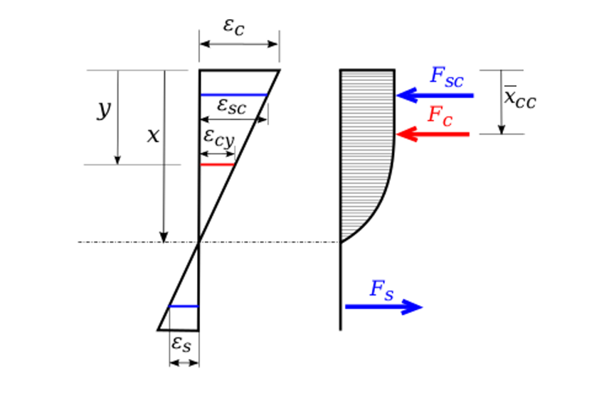
Figure 8. Deformations and stresses in compound bending

If domain 1: \({F}_{c}=0\)
If domain 2:

Since the section is partially compressed, the deformation in the concrete is given by:

\({\mathrm{\epsilon }}_{c}\left(y\right)=\left(\frac{{\mathrm{\epsilon }}_{c}}{x}\right)(x-y)\)

Being in PIVOT A, we have:

\({\mathrm{\epsilon }}_{c}=\frac{x}{x-d}\cdot {\mathrm{\epsilon }}_{\mathit{ud}}\)

So:

\({F}_{c}=b\underset{0}{\overset{x}{\int }}{\sigma }_{c}(y)\mathit{dy}=b\underset{0}{\overset{x}{\int }}{f}_{\mathit{cd}}(1-{(1-{\epsilon }_{c}(y)/{\epsilon }_{c2})}^{n})\mathit{dy},\mathit{si}{\epsilon }_{c}\le {\epsilon }_{c2}\) \({F}_{c}=b\underset{0}{\overset{x}{\int }}{\sigma }_{c}(y)\mathit{dy}=b\left[\underset{0}{\overset{\stackrel{´}{x}}{\int }}{f}_{\mathit{cd}}\left(1-{\left(1-{\epsilon }_{c}\left(y\right)/{\epsilon }_{c2}\right)}^{n}\right)\mathit{dy}+{f}_{\mathit{cd}}\left(x-\stackrel{´}{x}\right)\right],\mathit{si}{\mathrm{\epsilon }}_{c}\ge {\mathrm{\epsilon }}_{c2}\)

Where \(\stackrel{´}{x}\) corresponds to the limit between the elastic and plastic domain for concrete, such as \({\mathrm{\epsilon }}_{c}\left(\stackrel{´}{x}\right)={\mathrm{\epsilon }}_{c2}\), which is \(\stackrel{´}{x}=\left(\frac{{\mathrm{\epsilon }}_{c2}}{{\mathrm{\epsilon }}_{c}}\right)x\).

Finally, the thrust center of the \({F}_{c}\) effort is estimated as follows:

\({\stackrel{´}{x}}_{\mathit{cc}}=\frac{b\underset{0}{\overset{x}{\int }}{\sigma }_{c}\left(y\right)\mathrm{.}(\frac{h}{2}-y)\mathit{dy}}{{F}_{c}}\)

And as a result:

\({M}_{c}={F}_{c}\times {\stackrel{´}{x}}_{\mathit{cc}}\)

If domains 3 and 4:

Since the section is always partially compressed, the deformation in the concrete is always given by:

\({\mathrm{\epsilon }}_{c}\left(y\right)=\left(\frac{{\mathrm{\epsilon }}_{c}}{x}\right)y\)

Being in PIVOT B, we have:

\({\mathrm{\epsilon }}_{c}={\mathrm{\epsilon }}_{\mathit{cu}2}\)

So:

\({F}_{c}=b\underset{0}{\overset{x}{\int }}{\sigma }_{c}(y)\mathit{dy}=b\left[\underset{0}{\overset{\stackrel{´}{x}}{\int }}{f}_{\mathit{cd}}\left(1-{\left(1-{\epsilon }_{c}\left(y\right)/{\epsilon }_{c2}\right)}^{n}\right)\mathit{dy}+{f}_{\mathit{cd}}\left(x-\stackrel{´}{x}\right)\right]\)

Finally, we will always have:

\({\stackrel{´}{x}}_{\mathit{cc}}=\frac{b\underset{0}{\overset{x}{\int }}{\sigma }_{c}\left(y\right)\mathrm{.}(\frac{h}{2}-y)\mathit{dy}}{{F}_{c}}\)

And as a result:

\({M}_{c}={F}_{c}\times {\stackrel{´}{x}}_{\mathit{cc}}\)

If domain 5:

In this case, the section is entirely compressed, so that the diagram passes through the PIVOT C; this pivot being defined as being the intersection of the two deformation diagrams below:

Partially compressed case limit (PIVOT B with the neutral axis located at the bottom of the section)
Case of pure compression (\({\mathrm{\epsilon }}_{c}\left(y\right)={\mathrm{\epsilon }}_{c2}\) over the entire height of the section)

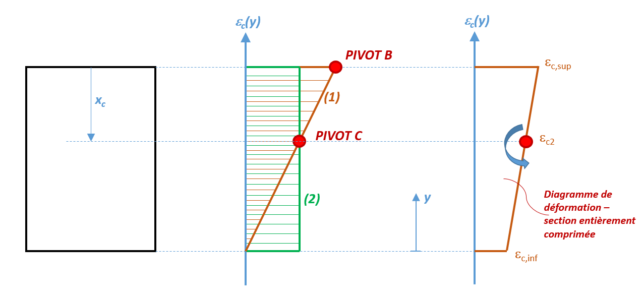
Figure 9. Construction of the PIVOT C from the two limit diagrams (1) and (2) .

So the depth of the PIVOT C will be evaluated at:

\({x}_{c}=\left(1-\frac{{\mathrm{\epsilon }}_{c2}}{{\mathrm{\epsilon }}_{\mathit{cu}2}}\right)h\)

Where \(h\) refers to the height of the section. In particular, the PIVOT C separates the two areas of the law of concrete behavior, so that:

\({\mathrm{\epsilon }}_{c}\left(C\right)={\mathrm{\epsilon }}_{c2}\)

Moreover, with the notations given in FIG. 9, the deformation diagram will be written:

\({\mathrm{\epsilon }}_{c}\left(y\right)=\frac{∆\mathrm{\epsilon }}{h}y+{\mathrm{\epsilon }}_{c,\mathit{inf}}\)

With:

\({\mathrm{\epsilon }}_{c}\left({y}_{c}\right)={\mathrm{\epsilon }}_{c}\left(h-{x}_{c}\right)=\frac{∆\mathrm{\epsilon }}{h}\left(h-{x}_{c}\right)+{\mathrm{\epsilon }}_{c,\mathit{inf}}={\mathrm{\epsilon }}_{c2}\)

So the main unknown of the problem in PIVOT C is \(∆\mathrm{\epsilon }\) (compared to \(x\) for the problem in PIVOT A or B), so that:

\({\mathrm{\epsilon }}_{\text{c,sup}}={\mathrm{\epsilon }}_{c,\mathit{inf}}+∆\mathrm{\epsilon }\)

The effort taken up by the concrete is then estimated as follows:

\({F}_{c}=b\underset{0}{\overset{h}{\int }}{\sigma }_{c}(y)\mathit{dy}=b\left[\underset{0}{\overset{h-{x}_{c}}{\int }}{f}_{\mathit{cd}}\left(1-{\left(1-{\epsilon }_{c}\left(y\right)/{\epsilon }_{c2}\right)}^{n}\right)\mathit{dy}+{f}_{\mathit{cd}}{x}_{c}\right]\)

Finally, the thrust center of the \({F}_{c}\) effort is estimated as follows:

\({\stackrel{´}{x}}_{\mathit{cc}}=\frac{b\underset{0}{\overset{h}{\int }}{\sigma }_{c}\left(y\right)\mathrm{.}(y-\frac{h}{2})\mathit{dy}}{{F}_{c}}\)

And as a result:

\({M}_{c}={F}_{c}\times {\stackrel{´}{x}}_{\mathit{cc}}\)

1.2.1.3. Difference between BAEL91 and EC2#

The flexure sizing algorithm composed in ELU presented in the previous paragraph is identical for both codifications, only a few input data are different. The table below summarises the differences between the two codifications currently used.

Coding:	BAEL91	EC2
parameters of the simplified rectangular concrete diagram	\(\mathrm{\lambda }=\mathrm{0,8}\)	\(\mathrm{\lambda }=\mathit{min}[0.8;0.8-\frac{{f}_{\mathit{ck}}-50}{400}]\)
parameters of the simplified rectangular concrete diagram	\(\mathrm{\eta }=1\)	\(\mathrm{\eta }=\mathit{min}[1;1-\frac{{f}_{\mathit{ck}}-50}{200}]\)
Design deformation limit of steels	\({\mathrm{\epsilon }}_{\mathit{ud}}=1\text{\%}\)	\({\mathrm{\epsilon }}_{\mathit{ud}}=0.9{\mathrm{\epsilon }}_{\mathit{uk}}\) where \({\mathrm{\epsilon }}_{\mathit{uk}}\) depends on the ductility class of the steels
design deformation in compression of concrete	\({\mathrm{\epsilon }}_{\mathit{cu}2}=\mathrm{0,35}\text{\%}\)	\({\mathrm{\epsilon }}_{\mathit{cu}2}(\text{\%})=\mathit{min}[0.35;0.26+3.5{(\frac{90-{f}_{\mathit{ck}}}{100})}^{4}]\)
Design deformation in compression of concrete in the frame of Pivot C	\({\mathrm{\epsilon }}_{c2}=\mathrm{0,2}\text{\%}\)	\({\epsilon }_{c2}(\text{‰})=\mathit{min}[\mathrm{2,0};2+0.085{({f}_{\mathit{ck}}-50)}^{0.53}]\)
concrete compression design stress	\({f}_{\mathit{cd}}=\frac{{\mathrm{\alpha }}_{\mathit{cc}}{f}_{\mathit{cj}}}{{\mathrm{\gamma }}_{c}}\) where \({\mathrm{\alpha }}_{\mathit{cc}}=\mathrm{0,85}\)	\({f}_{\mathit{cd}}=\frac{{\mathrm{\alpha }}_{\mathit{cc}}{f}_{\mathit{ck}}}{{\mathrm{\gamma }}_{c}}\) where \({\mathrm{\alpha }}_{\mathit{cc}}=1\)
design constraint of steels	\({f}_{\mathit{yd}}=\frac{{f}_{e}}{{\mathrm{\gamma }}_{s}}\)	\({f}_{\mathit{yd}}=\frac{{f}_{\mathit{yk}}}{{\mathrm{\gamma }}_{s}}\)

1.2.2. Calculation of longitudinal reinforcement in deflected flexure#

In this part, the section is subjected to both a bending moment along the Y axis and another along the Z axis, as well as to a normal force (positive under compression).

The case of deflected or compound-deflected flexure is more complex to solve. In fact, the interaction diagram (resistance limit surface) is in this case three-dimensional, in accordance with the figure below:

Figure 10. 3D interaction diagram along the N, My, Mz axes in the case of a deviated composite section

Consequently, an exact and rigorous dimensioning process (similar to the previous calculations in the documentation) would be complex to develop, as a result of this 3D reality of the stresses. In the current version of CALC_FERRAILLAGE of code_aster, we will therefore opt for a simplified verification procedure, for the moment.

In fact, it will be an “iterative” (and therefore non-deterministic) sizing method, based on the principle of verifying the Bresler inequality developed by Bresler, as presented in §5.8.9 of Eurocode 2. This method will thus make it possible to study separately, and in a perfectly decoupled manner, the two compound flexions stressing the section, the first (N, My) along the main axis of inertia Y and the second (N, Mz) following the second main axis of inertia, Z. Once the reinforcements have been obtained at the end of the calculations of sizing with respect to these two compound flexions (namely the Asy, Sup/asy quadruplet, InFy, /Asz, Sup/asz, inf), the method of dimensioning in deviated bending then consists in verifying the following inequality:

\({(\frac{{M}_{y}}{{M}_{\mathit{Ry}}})}^{a}+{(\frac{{M}_{z}}{{M}_{\mathit{Rz}}})}^{a}\le 1\)

Where the moments \({M}_{\mathit{Ry}}\) and \({M}_{\mathit{Rz}}\) are the moments of resistance in composite bending, under the normal force acting \(N\), of the reinforced section respectively along the Y axis (i.e. with the pair Asy, Sup/asy, inf) and along the Z axis (i.e. with the pair Asz, Sup/Asz, inf) and along the Z axis (i.e. with the pair Asz, Sup/Asz, inf). These moments of resistance are deduced from the “2D” interaction diagrams along Y and Z respectively.

The exponent \(a\) is calculated as a function of the ratio between the normal force \(N\) applying to the section, and the maximum normal resisting force, namely \({N}_{R}={A}_{c}\cdot {f}_{\mathit{cd}}+{A}_{s}\cdot {f}_{\mathit{yd}}\). In practice, \(a\) will be calculated by interpolation between the values given in the table in Figure below (as extracted from §5.8.9 of Eurocode 2); in particular, for \(N/{N}_{R}<0.1\), we will take \(a=1\).

N/N R	0.1	0.7	1
a	1	1.5	2

Figure 11. Calculation of the coefficient « a » for the Bresler method of EC2.

Thus, as long as the Bresler inequality is not verified (that is, if the sum of the left-hand side is greater than 1), the algorithm currently proposed in CALC_FERRAILLAGE will resume the calculation of the moments of resistance by proportionally increasing the four reinforcement sections as follows:

\({A}_{\text{sy,sup}}[i+1]={A}_{\text{sy,sup}}[i]\text{}+\text{}{\mathrm{\rho }}_{\text{sy,sup}}[i]\times {A}_{\text{s,iter}}[i]\)

\({A}_{\text{sy,inf}}[i+1]={A}_{\text{sy,inf}}[i]\text{}+\text{}{\mathrm{\rho }}_{\text{sy,inf}}[i]\times {A}_{\text{s,iter}}[i]\)

\({A}_{\text{sz,sup}}[i+1]={A}_{\text{sz,sup}}[i]\text{}+\text{}{\mathrm{\rho }}_{\text{sz,sup}}[i]\times {A}_{\text{s,iter}}[i]\)

\({A}_{\text{sz,inf}}[i+1]={A}_{\text{sz,inf}}[i]\text{}+\text{}{\mathrm{\rho }}_{\text{sz,inf}}[i]\times {A}_{\text{s,iter}}[i]\)

Such as:

\({\mathrm{\rho }}_{\text{sy,sup}}[i]={A}_{\text{sy,sup}}[i]/{A}_{\text{s,TOT}}[i]\)

\({\mathrm{\rho }}_{\text{sy,inf}}[i]={A}_{\text{sy,inf}}[i]/{A}_{\text{s,TOT}}[i]\)

\({\mathrm{\rho }}_{\text{sz,sup}}[i]={A}_{\text{sz,sup}}[i]/{A}_{\text{s,TOT}}[i]\)

\({\mathrm{\rho }}_{\text{sz,inf}}[i]={A}_{\text{sz,inf}}[i]/{A}_{\text{s,TOT}}[i]\)

With: \({A}_{\text{s,TOT}}[i]={A}_{\text{sy,sup}}[i]+{A}_{\text{sy,inf}}[i]+{A}_{\text{sz,sup}}[i]+{A}_{\text{sz,inf}}[i]\), and \({A}_{\text{s,iter}}[i]\) denotes an iteration section (currently taken by default) equal to 10% of \({A}_{\text{s,TOT}}[i]\).

1.2.3. Calculation of transverse reinforcement#

The first step is to define the transverse reinforcement ratio in accordance with the following expression:

\({\rho }_{w}=\frac{{A}_{\mathit{sw}}}{s{b}_{w}\mathrm{sin}(\alpha )}\)

Where:

\({A}_{\mathit{sw}}\) refers to the total cross-sectional area (per reinforcement plane) of the transverse reinforcements.
\(s\) refers to the longitudinal spacing between transverse reinforcement frames.
\({b}_{w}\) refers to the smallest width of the stretched area of the element’s cross section.
\(\alpha\) refers to the angle of inclination of the transverse reinforcement frames with respect to the longitudinal axis of the element.

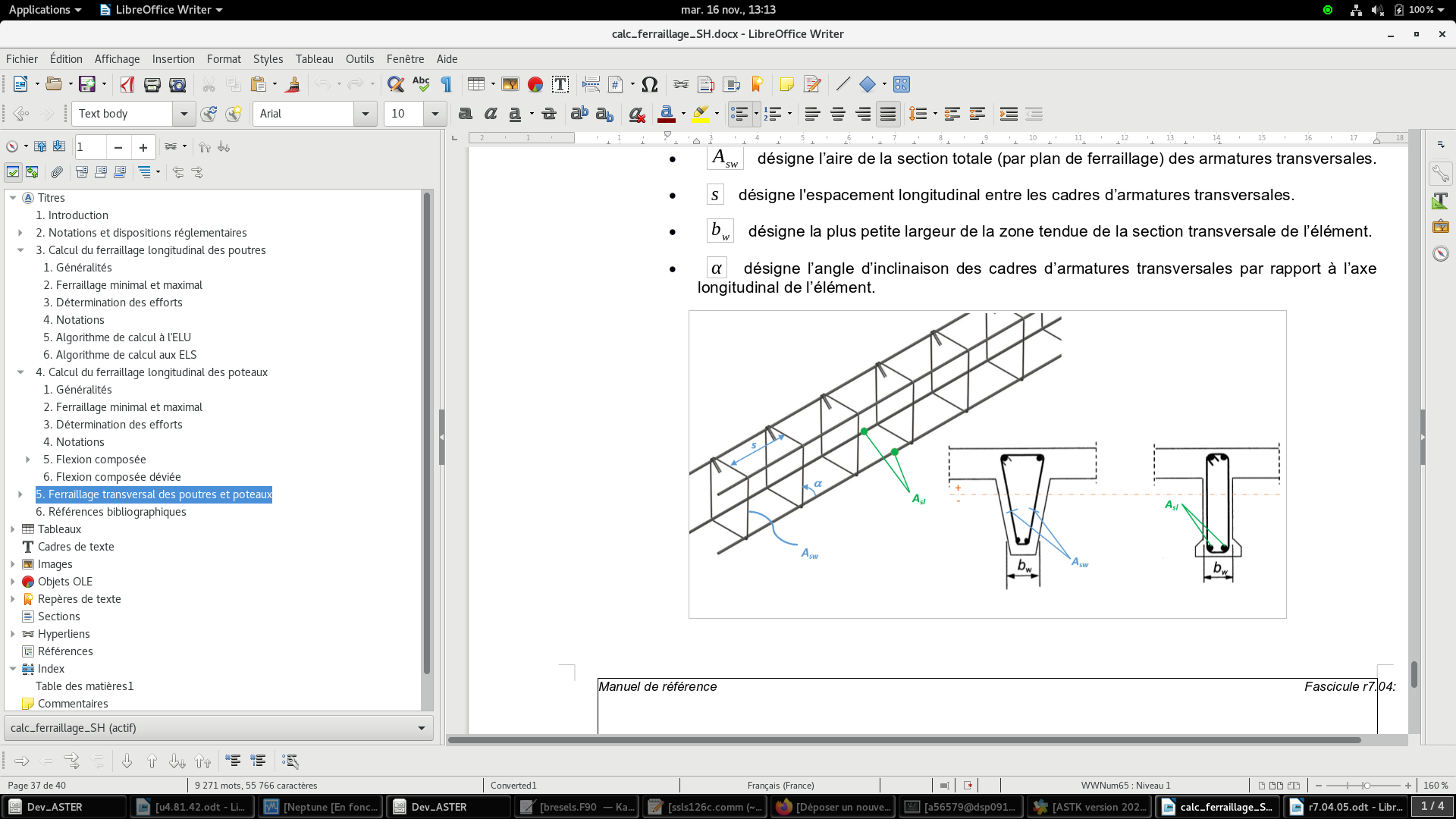
Figure 12. Transverse reinforcement of a 1D element (beam or column)

In addition, for the time being, the following hypotheses will be made:

the frames will be assumed to be straight, which is equivalent to asking \(\alpha =90°\), which is \(\mathrm{sin}(\alpha )=1\).
the elements considered are rectangular in cross section, and therefore \({b}_{w}=b\).

The cross section is thus subjected to a cutting force \({V}_{\mathit{Ed}}\), as well as to a torsional moment \({T}_{\mathit{Ed}}\).

By default, no transverse reinforcement is required as long as the previous couple of stresses does not exceed the shear strength capacities of concrete alone; this therefore amounts to verifying the following inequality:

\(\frac{{V}_{\mathit{Ed}}}{{V}_{\mathit{Rd},c}}+\frac{{T}_{\mathit{Ed}}}{{T}_{\mathit{Rd},c}}⩽1\)

Such as:

\({V}_{\mathit{Rd},c}=[\mathit{max}({C}_{\mathit{Rd},c}k{(100{\mathrm{\rho }}_{l}{f}_{\mathit{ck}})}^{1/3};{v}_{\mathit{min}})+{k}_{1}{\mathrm{\sigma }}_{\mathit{cp}}]\times {b}_{w}d\)
\({T}_{\mathit{Rd},c}=2{f}_{\mathit{ctd}}{t}_{k}{A}_{k}\)

Where:

\({f}_{\mathit{ck}}\) in MPa
\({C}_{\mathit{Rd},c}=\mathrm{0,18}/{\mathrm{\gamma }}_{c}\)
\(k=1+\sqrt{\frac{200}{d}}⩽\mathrm{2,0}\), with “d” in mm
\({\mathrm{\rho }}_{l}=\frac{{A}_{\mathit{sl}}}{{b}_{w}d}⩽\mathrm{0,02}\), where Asl represents the section of the tensile reinforcements (resulting from the composite bending calculation)
\({v}_{\mathit{min}}=\raisebox{1ex}{\mathrm{0,053}}\!\left/ \!\raisebox{-1ex}{{\mathrm{\gamma }}_{c}}\right.\times {k}^{\mathrm{1,5}}\times {f}_{\mathit{ck}}^{\mathrm{0,5}}\), in the case of beams
\({k}_{1}=\mathrm{0,15}\)
\({\mathrm{\sigma }}_{\mathit{cp}}=\frac{{N}_{\mathit{Ed}}}{{b}_{w}h}⩾0\), where NEdreprésente the normal force (positive in compression)
\({f}_{\mathit{ctd}}={f}_{\mathit{ctk}}/{\mathrm{\gamma }}_{c}\), where fctk represents the tensile strength of concrete, such as \({f}_{\mathit{ctk}}=\begin{array}{c}\mathrm{0,7}\times \mathrm{0,3}\times {f}_{\mathit{ck}}^{2/3},\text{si}{f}_{\mathit{ck}}⩽50\mathit{MPa}\\ \mathrm{0,7}\times \mathrm{2,12}\times \mathrm{log}(1+\mathrm{0,1}\times ({f}_{\mathit{ck}}+8)),\text{si}{f}_{\mathit{ck}}⩾50\mathit{MPa}\end{array}\)
\({t}_{k}=\mathit{max}[{b}_{w}h/(2\times ({b}_{w}+h));2{c}_{\text{sup}};2{c}_{\text{inf}}]\)
\({A}_{k}=({b}_{w}-{t}_{k})\times (h-{t}_{k})\)

In the opposite case, i.e. in the case where the left member of the previous inequality is greater than 1, the dimensioning of transversal shear reinforcement is based on a Ritter-Mörsh lattice model formed by a coupling between compression rods — which represent the portion of concrete resistant to shear — and the transverse reinforcement frames. This lattice is schematized in the following figure, whose notations are explained below.

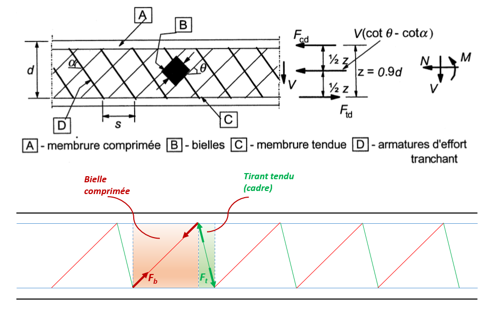
Figure 13. Tie rod structure for beams subjected to shear stress

\(\alpha\) is the angle between the shear reinforcements and the average fiber of the element. (As a reminder, we will consider \(\alpha =90°\) in algorithm).
\(\theta\) is the angle between the compression rod and the average fiber of the element. In accordance with Eurocode 2 regulations, the value of \(\theta\) must respect the \(1\le \mathit{cot\theta }\le \mathrm{2,5}\) domain.
\({F}_{\mathit{td}}\) is the calculation value of the tensile force taken up by the lower tensile longitudinal reinforcements.
\({F}_{\mathit{cd}}\) is the calculation value of the compression force taken up by the height of compressed concrete (as a function of the depth of the neutral axis, as determined at the end of the composite bending calculation), as well as the possible upper compression reinforcement.
\({b}_{w}\) is the smallest width of the section between the stretched chord and the compressed chord. In the calculation algorithm, we will therefore use \({b}_{w}=b\).
\(z\) is the lever arm for the internal forces, for an element of constant height, corresponding to the bending moment in the element in question. For shear force calculations of a partially compressed reinforced concrete section (neutral axis within the section), the calculation algorithm will consider as value:

\(z=({F}_{s,s}{z}_{1}+{F}_{\mathit{cc}}{z}_{1})/({F}_{s,s}+{F}_{\mathit{cc}})\)

Such that \({z}_{1}=h-{c}_{\text{inf}}-{c}_{\text{sup}}\) represents the lever arm of the upper compressed reinforcements compared to the center of gravity of the lower tension reinforcements, and \({z}_{2}=(1-\mathrm{0,5}\mathrm{\lambda }\mathrm{\alpha })\times d\) represents the lever arm of the center of gravity of the compressed concrete height with respect to the center of gravity of the compressed concrete with respect to the center of gravity of the lower tensile reinforcements. \({F}_{s,s}={A}_{\text{s,s}}{\mathrm{\sigma }}_{\text{s,s}}\) represents the force taken up by the compressed reinforcements and \({F}_{\mathit{cc}}=\mathrm{\eta }\mathrm{\lambda }\times \mathrm{\alpha }\times \mathit{bd}{f}_{\mathit{cd}}\) represents the force taken up by the height of compressed concrete.

For other cases, we can adopt the approximate value \(z=\mathrm{0,9}d\)

The mesh thus modelled will withstand the demanding shear force, diagonal by diagonal, as follows:

on the one hand, the compression rod (compressed diagonal), whose resistance is given by:

\({V}_{\mathit{Rd},\mathit{max}}={\alpha }_{\mathit{cw}}{b}_{w}z{\nu }_{1}{f}_{\mathit{cd}}\frac{(\mathrm{cot}\mathrm{\theta }+\mathrm{cot}\mathrm{\alpha })}{1+{\mathrm{cot}}^{2}\mathrm{\theta }}\), with respect to the shear force

\({T}_{\mathit{Rd},\mathit{max}}=2{\alpha }_{\mathit{cw}}{\nu }_{1}{f}_{\mathit{cd}}{A}_{k}{t}_{k}\mathrm{sin}\mathrm{\theta }\mathrm{cos}\mathrm{\theta }\), with respect to the moment of twisting

It will therefore be necessary to verify, for the inclination of the rod in question, the following inequality:

\(\frac{{V}_{\mathit{Ed}}}{{V}_{\mathit{Rd},\mathit{max}}}+\frac{{T}_{\mathit{Ed}}}{{T}_{\mathit{Rd},\mathit{max}}}⩽1\)

on the other hand, the frame (stretched/pulling diagonal), whose resistance is given by:

\({V}_{\mathit{Rd},s}=\frac{{A}_{\mathit{sw}}}{s}z{f}_{\mathit{ywd}}(\mathrm{cot}\mathrm{\theta }+\mathrm{cot}\mathrm{\alpha })\mathrm{sin}\mathrm{\alpha }\)

Where:

\({f}_{\mathit{ywd}}\) is the design elastic limit of shear reinforcements (taken equal to \({f}_{\mathit{yd}}\))
\({\nu }_{1}=\nu =\mathrm{0,6}(1-\frac{{f}_{\mathit{ck}}}{250})\), with \({f}_{\mathit{ck}}\) in MPa, is a coefficient for reducing the shear strength of cracked concrete
\({\alpha }_{\mathit{cw}}\) is a coefficient taking into account the stress state in the compressed chord, and whose value varies according to the average compression stress \({\mathrm{\sigma }}_{\mathit{cp}}\) taken up by the compressed concrete, such as:

\({\alpha }_{\mathit{cw}}=1\) for structures that are not prestressed and not subject to compression stress

\({\alpha }_{\mathit{cw}}=1+\frac{{\mathrm{\sigma }}_{\mathit{cp}}}{{f}_{\mathit{cd}}}\), for \(0<{\mathrm{\sigma }}_{\mathit{cp}}\le 0.25{f}_{\mathit{cd}}\)

\({\alpha }_{\mathit{cw}}=1.25\), for \(0.25{f}_{\mathit{cd}}<{\mathrm{\sigma }}_{\mathit{cp}}\le 0.5{f}_{\mathit{cd}}\)
\({\alpha }_{\mathit{cw}}=2.5(1-\frac{{\mathrm{\sigma }}_{\mathit{cp}}}{{f}_{\mathit{cd}}})\), for \(0.5{f}_{\mathit{cd}}<{\mathrm{\sigma }}_{\mathit{cp}}\le {f}_{\mathit{cd}}\)

The principle of dimensioning transverse reinforcement then consists in equating the term \({V}_{\mathit{Rd},s}\) to the shear force stressing the section, given as follows:

\({V}_{\mathit{Rd},s}={V}_{\mathit{Ed}}+({T}_{\mathit{Ed}}/{A}_{k})\times (h-{t}_{k})\)

It will then be a question of choosing the value of θ allowing to minimize the ASW/s density, while verifying the inequality of not crushing the connecting rods.

1.2.4. Impact of shear forces on longitudinal reinforcement#

In accordance with the specifications of Eurocode 2, and in the case where transverse reinforcement is required as a result of the calculation carried out in the previous paragraph, the additional tensile force ΔFtD induced in the longitudinal reinforcements and due to the shear force VEd and to the torsional moment TEd, is written as follows:

\(\mathrm{\Delta }{F}_{\mathit{td}}={V}_{\mathit{Ed}}\mathrm{cot}\mathrm{\theta }+{T}_{\mathit{Ed}}\mathrm{cot}\mathrm{\theta }\times ({u}_{k}/2{A}_{k})\)

Or θ designates the angle of inclination of the links of the truss, as retained in the preceding dimensioning. The current version of the code_aster CALC_FERRAILLAGE operator offers the possibility of taking into account this additional traction effort; for this reason, all you have to do is take EPURE_CISA = “OUI”.

1.3. Sizing to the ELS Feature#

1.3.1. Calculation of longitudinal reinforcement in simple or compound bending#

In the case of the calculation at ELS, a homogenized steel-concrete section is considered, so that the stress diagram is systematically linear.

For the following, the quantities are defined below:

{\({\epsilon }_{c},{\sigma }_{c}\}\) respectively the deformation and the stress experienced at the level of the most compressed concrete fiber. In accordance with the above (linear stress diagram), we have \({\sigma }_{c}={E}_{c}{\epsilon }_{c}\), such as \({\epsilon }_{c}>0\) in compression.
{\({\epsilon }_{s},{\sigma }_{s}\}\) respectively the deformation and the stress experienced under tension steel, such as \({\sigma }_{s}={E}_{s}{\epsilon }_{s}\) and \({\epsilon }_{s}<0\) under tension.

In accordance with the notations in the following figure, the resultant of the compressive stresses in concrete is equal, for the partially compressed case:

\({F}_{c}=\frac{1}{2}{\sigma }_{c}\mathit{bx}=\frac{1}{2}{E}_{c}{\epsilon }_{c}\mathit{bx}\)

In accordance with the linearity of the stress diagram, and always in the case of a partially compressed section, this force is applied at a distance \(\frac{x}{3}\) from the most compressed fiber of the concrete, i.e. at a distance \(\left(d-\frac{x}{3}\right)\) from the main longitudinal steel (or \(\left(d\text{'}-\frac{x}{3}\right)\) if the stress moment is negative).

Moreover, the force experienced by the tensile steel is equal to:

\({F}_{s}={A}_{s}{\sigma }_{s}={A}_{s}{E}_{s}{\epsilon }_{s}\)

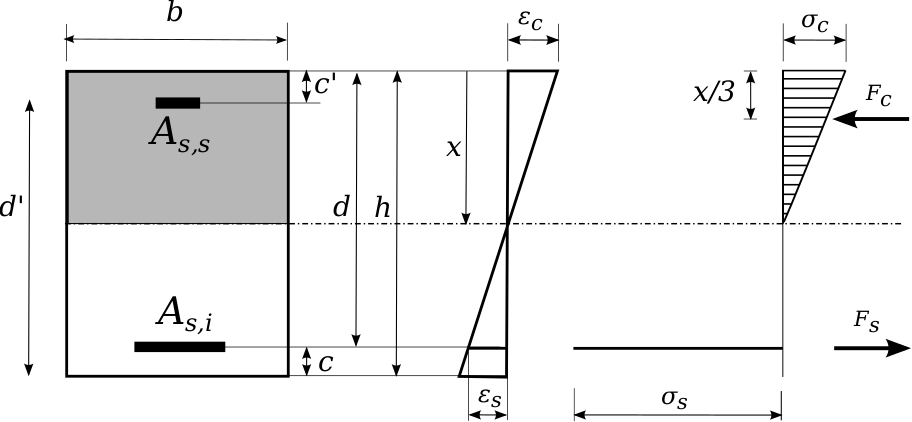
Figure 14. Resulting stresses and forces on a reinforced concrete section subjected to flexural stress composed of ELS

In the description of the algorithm that follows, the bending moment and the normal effort at ELS requesting the section, namely \({M}_{\mathit{cara}},{N}_{\mathit{cara}}\), will be noted \(M,N\) in order to simplify writing.

In a manner similar to the dimensioning in ELU, the aim is to express the demanding moment at the center of gravity of the tension reinforcements, such as:

\({M}_{\mathit{inf}}=M+N\cdot \left(\frac{h}{2}-c\right),\mathit{si}M>0\)

\({M}_{\text{sup}}=-M+N\cdot \left(\frac{h}{2}-{c}^{\text{'}}\right),\mathit{si}M<0\)

We will now continue with the case M>0 (the other case is obtained symmetrically).

From the linearity of the stress diagram, and by setting \(x=\xi \cdot d\), the relationship between the stress in tension steel and that in the right of compressed concrete is written:

\({\sigma }_{s}=\frac{1-\xi }{\xi }{\alpha }_{e}{\sigma }_{c}\)

Where \({\alpha }_{e}=\frac{{E}_{s}}{{E}_{c}}\) refers to the ratio between the Young’s modulus of steel and that of concrete (making it possible to obtain a homogenized cross section).

The balance of moments is then written as:

\({M}_{\mathit{inf}}={F}_{c}\cdot {z}_{c}=\left(\frac{1}{2}\mathit{bx}{\sigma }_{c}\right)\cdot \left(d-\frac{x}{3}\right)\)

Reduced moments can be defined as follows:

\({\mu }_{\mathit{inf}}=\frac{{M}_{\mathit{inf}}}{b{d}^{2}{\sigma }_{c,\text{lim}}}\)

Where \({\sigma }_{c,\text{lim}}\) is the limit stress that compressed concrete can take up at the ELS characteristic.

The previous balance is then rewritten as follows:

\({\mu }_{\mathit{inf}}=\frac{1}{2}\xi \left(1-\frac{\xi }{3}\right)\frac{{\sigma }_{c}}{{\sigma }_{c,\text{lim}}}\)

On the other hand, the balance of forces is written (considering only lower steel):

\(N={F}_{c}+{F}_{s}=\frac{1}{2}\mathit{bx}{\sigma }_{c}+{A}_{s,i}\cdot {\sigma }_{s,i}\)

Similar to the pivot rule in the deformation graph in ELU, the service-limit state of the section can be reached using similar pivots but on the stress graph, either on the steel side for \({\sigma }_{s}={\sigma }_{s,\text{lim}}\), or on the compressed concrete side for \({\sigma }_{c}={\sigma }_{c,\text{lim}}\). By gradually increasing the value of \(\xi\) — neutral axis depth coefficient such as \(\xi =\frac{x}{d}\) — the stress diagram starts by « pivoting » around the pivot relative to the tension steel limit (\({\sigma }_{s}={\sigma }_{s,\text{lim}}\)), and then « pivoting » around the pivot relative to the limit of compressed concrete (\({\sigma }_{c}={\sigma }_{c,\text{lim}}\)). In this sense, the limit separating the two « pivoting » zones is obtained by simultaneously saturating the two constraint limitation criteria, namely by having both \({\sigma }_{c}={\sigma }_{c,\text{lim}}\) and \({\sigma }_{s}={\sigma }_{s,\text{lim}}\); we then obtain:

\({\xi }_{\mathrm{1,2}}=\frac{{\alpha }_{e}{\sigma }_{c,\text{lim}}}{{\alpha }_{e}{\sigma }_{c,\text{lim}}+{\sigma }_{s,\text{lim}}}\)

By then referring to the equation of the reduced moment given in the above, we then calculate the limited reduced moment \({\stackrel{´}{\mu }}_{\text{inf}}\) (or \({\stackrel{´}{\mu }}_{\text{sup}}\) if M < 0), obtained for \({\xi =\xi }_{\mathrm{1,2}}\), making it possible to recognize the pivot to be retained for a given pair (M, N). Thus, in the case where M > 0:

If \({\mu }_{\text{inf}}<{\stackrel{´}{\mu }}_{\text{inf}}\), it is the pivot relating to the tension steel that is used, namely \({\sigma }_{s}={\sigma }_{s,\text{lim}}\).

In this case, the relationships given then make it possible to express the stress to the right of the most compressed concrete fiber \({\sigma }_{c}\), as a function of \({\sigma }_{s,\text{lim}}\), \({\mathrm{\alpha }}_{e}\) and \(\xi\). The balance of moments is then rewritten as follows:

\(\frac{1}{2}\frac{{\sigma }_{s,\text{lim}}}{{\alpha }_{e}{\sigma }_{c,\text{lim}}}\frac{{\xi }^{2}}{1-\xi }(1-\frac{\xi }{3})={\mu }_{\mathit{inf}}\)

Solving this 3rd degree polynomial equation makes it possible to determine the depth coefficient of the neutral axis \(\xi\); from there, the equation for the balance of normal forces then makes it possible to calculate the main steel section \({A}_{s}\).

If \({\mu }_{\text{inf}}>{\stackrel{´}{\mu }}_{\text{inf}}\), it is the pivot relating to compressed concrete that is used, namely \({\sigma }_{c}={\sigma }_{c,\text{lim}}\).

The balance of moments given above is then rewritten as follows:

\({\mu }_{\mathit{inf}}=\frac{1}{2}\xi (1-\frac{\xi }{3})\)

The resolution of this 2nd degree polynomial equation makes it possible to determine the depth coefficient of the neutral axis \(\xi\); from there, we determine the stress at the right of the \({\sigma }_{s}\) tension steel, and this as a function of \({\sigma }_{c,\text{lim}}\), \({\mathrm{\alpha }}_{e}\) and \(\xi\). The equation for the balance of normal forces then makes it possible to calculate the main steel section \({A}_{s}\).

If the previous balance results in a negative value of \({A}_{s}\), or if we find ourselves in an entirely tense or fully compressed case, then the algorithm activates the keyword COND_ITER = VRAI.

For cases where COND_ITER = VRAI, it is then a question of scanning the different balance domains, that is to say by iterating \(\xi\) from -∞ to +∞. Based on the two equilibrium equations (moments and forces), the associated pair (As, s, As, i) is determined for each value of \(\xi\). The algorithm will finally retain the configuration resulting in a minimization of the sum As, S+as, i, while ensuring that both sections are positive.

So, by always having \(\xi =\frac{x}{d}\), \(\mathrm{\delta }=\frac{d}{h}\) and \(\mathrm{\delta }\text{'}=\frac{d\text{'}}{h}\), we can distinguish the cases below:

for \(\xi \le 0\), the section is fully stretched such that the stress diagram passes through the pivot relative to the main tensile steel (\({\sigma }_{s}=-{\sigma }_{\text{s,lim}}\)), with:
\({\sigma }_{c}=0\) (concrete has no resistance and in particular \({F}_{c}=0\))
\({\sigma }_{\mathit{sc}}=\frac{1-\delta \text{'}-\xi \cdot \mathrm{\delta }}{\mathrm{\delta }-\xi \cdot \mathrm{\delta }}{\sigma }_{s}\) (\({\sigma }_{\mathit{sc}}\) becomes negative, being a traction state, in accordance with the above).
for \(0<\xi <\frac{{\alpha }_{e}{\sigma }_{c,\text{lim}}}{{\alpha }_{e}{\sigma }_{c,\text{lim}}+{\sigma }_{s,\text{lim}}}\), the section is partially compressed such that the stress diagram always passes through the pivot relative to the main tension steel (\({\sigma }_{s}=-{\sigma }_{\text{s,lim}}\)), with:
\({\sigma }_{c}=\frac{\xi }{1-\xi }\frac{{\sigma }_{s,\text{lim}}}{{\alpha }_{e}}\)
\({\sigma }_{\mathit{sc}}=\frac{1-\delta \text{'}-\xi \cdot \mathrm{\delta }}{\mathrm{\delta }-\xi \cdot \mathrm{\delta }}{\sigma }_{s}\)
for \(\xi >\frac{{\alpha }_{e}{\sigma }_{c,\text{lim}}}{{\alpha }_{e}{\sigma }_{c,\text{lim}}+{\sigma }_{s,\text{lim}}}\), the section is partially compressed such that the stress diagram now passes through the pivot relating to the most compressed concrete fiber (\({\sigma }_{c}={\sigma }_{\text{c,lim}}\)), with:
\({\sigma }_{s}=\frac{\xi -1}{\xi }{\alpha }_{e}{\sigma }_{c,\text{lim}}\)
\({\sigma }_{\mathit{sc}}=\frac{\xi \cdot \mathrm{\delta }-1+\delta \text{'}}{\xi \cdot \mathrm{\delta }}{\alpha }_{e}{\sigma }_{c,\text{lim}}\)

For \(\xi =\frac{{\alpha }_{e}{\sigma }_{c,\text{lim}}}{{\alpha }_{e}{\sigma }_{c,\text{lim}}+{\sigma }_{s,\text{lim}}}\), the criterion is achieved simultaneously on the steel and concrete side.

Solving the two equilibrium equations (efforts and moments) will make it possible to determine the two unknowns of the problem, namely \({A}_{s,s}\) and \({A}_{s,i}\).

In the case where the section is completely compressed (neutral axis outside the section):

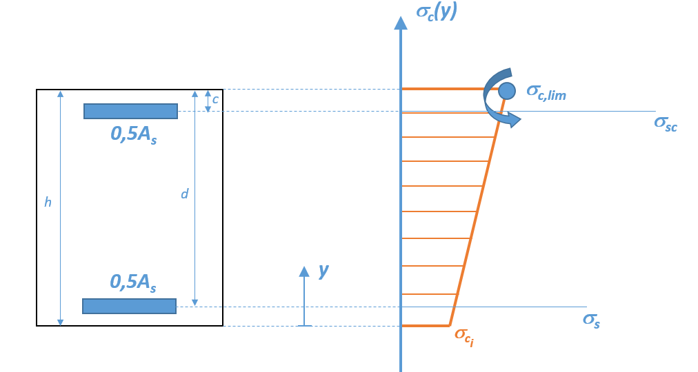
Figure 15. Bending stress diagram composed in ELS — fully compressed case.

Continuing with the previous case (\(\xi >\frac{{\alpha }_{e}{\sigma }_{c,\text{lim}}}{{\alpha }_{e}{\sigma }_{c,\text{lim}}+{\sigma }_{s,\text{lim}}}\)), the stress diagram always passes through the pivot relating to the most compressed concrete fiber (\({\sigma }_{c}={\sigma }_{\text{c,lim}}\)), with, in accordance with the notations in FIG. 13:

\(∆\mathrm{\sigma }={\mathrm{\sigma }}_{\text{c,lim}}-{\mathrm{\sigma }}_{{c}_{i}}\)
\({\mathrm{\sigma }}_{c}\left(y\right)={\mathrm{\sigma }}_{{c}_{i}}+(\frac{∆\mathrm{\sigma }}{h})y\)
\(\mathrm{\delta }=\frac{d}{h}\) and \(\mathrm{\delta }\text{'}=\frac{d\text{'}}{h}\)
\({\mathrm{\sigma }}_{\mathit{sc}}={\mathrm{\alpha }}_{e}({\mathrm{\sigma }}_{{c}_{i}}+∆\mathrm{\sigma }\cdot \mathrm{\delta }\text{'})\)
\({\mathrm{\sigma }}_{\mathit{sc}}={\mathrm{\alpha }}_{e}({\mathrm{\sigma }}_{{c}_{i}}+∆\mathrm{\sigma }\cdot (1-\mathrm{\delta }))\)

By setting \(X=\frac{∆\mathrm{\sigma }}{{\mathrm{\sigma }}_{\text{c,lim}}}\), the efforts taken up by the concrete of the section are written as follows:

Resisting effort: \({F}_{c}=\frac{1}{2}\mathit{bh}\left(2-X\right){\sigma }_{c,\text{lim}}\)
Resisting moment with respect to the center of the section: \({M}_{c}=\frac{1}{12}b{h}^{2}X{\sigma }_{c,\text{lim}}\)

The normal resisting force is then written as follows:

\({N}_{R}={F}_{c}+{F}_{\mathit{sc}}+{F}_{s}={F}_{c}+{A}_{s,s}{\mathrm{\sigma }}_{s,s}+{A}_{s,i}{\mathrm{\sigma }}_{s,i}\)

And the resisting moment (calculated at the center of the section) is written as follows:

\({M}_{R}={M}_{c}+{F}_{\mathit{sc}}\cdot (d\text{'}-\frac{h}{2})-{F}_{\mathit{sc}}\cdot (d-\frac{h}{2})\)

Solving the two equilibrium equations (efforts and moments) will make it possible to determine the two unknowns of the problem, namely \({A}_{s,s}\) and \({A}_{s,i}\).

1.3.2. Calculation of longitudinal reinforcement in deflected flexure#

Similar to the case in ELU (§1.2.2), it will be a question of applying an “iterative” (and therefore non-deterministic) sizing method, based on the principle of verifying the Bresler inequality developed by Bresler, as presented in §5.8.9 of Eurocode 2. This method will thus make it possible to study separately, and in a perfectly decoupled manner, the two compound flexions stressing the section, the first (N, My) along the main axis of inertia Y and the second (N, Mz) following the second main axis of inertia, Z. Once the reinforcements have been obtained at the end of the calculations of sizing with respect to these two compound flexions (namely the Asy, Sup/asy quadruplet, INF /Asz, Sup/asz, inf), the method of dimensioning in deviated bending then consists in verifying the following inequality:

\({(\frac{{M}_{y}}{{M}_{\mathit{Ry}}})}^{a}+{(\frac{{M}_{z}}{{M}_{\mathit{Rz}}})}^{a}\le 1\)

\({f}_{c}=\raisebox{1ex}{1}\!\left/ \!\raisebox{-1ex}{4}\right.\cdot ({\mathrm{\sigma }}_{c,\mathit{max}}^{\text{y,sup}}+{\mathrm{\sigma }}_{c,\mathit{max}}^{\text{y,inf}}+{\mathrm{\sigma }}_{c,\mathit{max}}^{\text{z,sup}}+{\mathrm{\sigma }}_{c,\mathit{max}}^{\text{z,inf}})\)

\({f}_{s}={\mathrm{\sigma }}_{s,\mathit{max}}\)

The rest of the sizing process is similar to that documented in ELU (see §1.2.2)

1.3.3. Calculation of transverse reinforcement#

The first step is to define the transverse reinforcement ratio in accordance with the following expression:

\({\rho }_{w}=\frac{{A}_{\mathit{sw}}}{s{b}_{w}\mathrm{sin}(\alpha )}\)

Where:

\({A}_{\mathit{sw}}\) refers to the total cross-sectional area (per reinforcement plane) of the transverse reinforcements.
\(s\) refers to the longitudinal spacing between transverse reinforcement frames.
\({b}_{w}\) refers to the smallest width of the stretched area of the element’s cross section.
\(\alpha\) refers to the angle of inclination of the transverse reinforcement frames with respect to the longitudinal axis of the element.

In addition, for the time being, the following hypotheses will be made:

the frames will be assumed to be straight, which is equivalent to asking \(\alpha =90°\), which is \(\mathrm{sin}(\alpha )=1\).
the elements considered are rectangular in cross section, and therefore \({b}_{w}=b\).

The cross section is thus subjected to a cutting force \({V}_{\mathit{cara}}\), as well as to a torsional moment \({T}_{\mathit{cara}}\).

\(\frac{{V}_{\mathit{cara}}}{{V}_{\mathit{Rd},c}}+\frac{{T}_{\mathit{cara}}}{{T}_{\mathit{Rd},c}}⩽1\)

Such as:

\({V}_{\mathit{Rd},c}=[\mathit{max}({C}_{\mathit{Rd},c}k{(100{\mathrm{\rho }}_{l}{f}_{\mathit{ck}})}^{1/3};{v}_{\mathit{min}})+{k}_{1}{\mathrm{\sigma }}_{\mathit{cp}}]\times {b}_{w}d\)
\({T}_{\mathit{Rd},c}=2{f}_{\mathit{ctd}}{t}_{k}{A}_{k}\)

Where:

\({f}_{\mathit{ck}}\) in MPa
\({C}_{\mathit{Rd},c}=\mathrm{0,18}/{\mathrm{\gamma }}_{c}\); \({\mathrm{\gamma }}_{c}={f}_{\mathit{ck}}/{\mathrm{\sigma }}_{c\mathrm{,0}}\), such as \({\mathrm{\sigma }}_{c\mathrm{,0}}=\raisebox{1ex}{1}\!\left/ \!\raisebox{-1ex}{2}\right.\cdot ({\mathrm{\sigma }}_{c,\mathit{max}}^{\text{sup}}+{\mathrm{\sigma }}_{c,\mathit{max}}^{\text{inf}})\)
\(k=1+\sqrt{\frac{200}{d}}⩽\mathrm{2,0}\), with “d” in mm
\({\mathrm{\rho }}_{l}=\frac{{A}_{\mathit{sl}}}{{b}_{w}d}⩽\mathrm{0,02}\), where Asl represents the section of the tensile reinforcements (resulting from the composite bending calculation)
\({v}_{\mathit{min}}=\raisebox{1ex}{\mathrm{0,053}}\!\left/ \!\raisebox{-1ex}{{\mathrm{\gamma }}_{c}}\right.\times {k}^{\mathrm{1,5}}\times {f}_{\mathit{ck}}^{\mathrm{0,5}}\), in the case of beams
\({k}_{1}=\mathrm{0,15}\)
\({\mathrm{\sigma }}_{\mathit{cp}}=\frac{{N}_{\mathit{cara}}}{{b}_{w}h}⩾0\), where Ncara represents the normal effort (positive in compression)
\({f}_{\mathit{ctd}}={f}_{\mathit{ctk}}/{\mathrm{\gamma }}_{c}\), where fctk represents the tensile strength of concrete, such as \({f}_{\mathit{ctk}}=\begin{array}{c}\mathrm{0,7}\times \mathrm{0,3}\times {f}_{\mathit{ck}}^{2/3},\text{si}{f}_{\mathit{ck}}⩽50\mathit{MPa}\\ \mathrm{0,7}\times \mathrm{2,12}\times \mathrm{log}(1+\mathrm{0,1}\times ({f}_{\mathit{ck}}+8)),\text{si}{f}_{\mathit{ck}}⩾50\mathit{MPa}\end{array}\)
\({t}_{k}=\mathit{max}[{b}_{w}h/(2\times ({b}_{w}+h));2{c}_{\text{sup}};2{c}_{\text{inf}}]\)
\({A}_{k}=({b}_{w}-{t}_{k})\times (h-{t}_{k})\)

\(\alpha\) is the angle between the shear reinforcements and the average fiber of the element. (As a reminder, we will consider \(\alpha =90°\) in algorithm).
\(\theta\) is the angle between the compression rod and the average fiber of the element. In accordance with Eurocode 2 regulations, the value of \(\theta\) must respect the \(1\le \mathit{cot\theta }\le \mathrm{2,5}\) domain.
\({b}_{w}\) is the smallest width of the section between the stretched chord and the compressed chord. In the calculation algorithm, we will therefore use \({b}_{w}=b\).
\(z\) is the lever arm for the internal forces, for an element of constant height, corresponding to the bending moment in the element in question. For shear force calculations of a partially compressed reinforced concrete section (neutral axis within the section), the calculation algorithm will consider as value:

\(z=({F}_{s,s}{z}_{1}+{F}_{\mathit{cc}}{z}_{1})/({F}_{s,s}+{F}_{\mathit{cc}})\)

Such that \({z}_{1}=h-{c}_{\text{inf}}-{c}_{\text{sup}}\) represents the lever arm of the upper compressed reinforcements compared to the center of gravity of the lower tension reinforcements, and \({z}_{2}=(1-\xi /3)\times d\) represents the lever arm of the center of gravity of the compressed concrete height with respect to the center of gravity of the compressed concrete with respect to the center of gravity of the lower tensile reinforcements. \({F}_{s,s}={A}_{\text{s,s}}{\mathrm{\sigma }}_{\text{s,s}}\) represents the force taken up by the compressed reinforcements and \({F}_{\mathit{cc}}=\mathrm{0,5}\times {\mathrm{\sigma }}_{\text{c,sup}}\mathit{\xi d}{b}_{w}\) represents the force taken up by the height of compressed concrete.

For other cases, we can adopt the approximate value \(z=\mathrm{0,9}d\)

The mesh thus modelled will withstand the demanding shear force, diagonal by diagonal, as follows:

on the one hand, the compression rod (compressed diagonal), whose resistance is given by:

\({V}_{\mathit{Rd},\mathit{max}}={\alpha }_{\mathit{cw}}{b}_{w}z{\nu }_{1}{\mathrm{\sigma }}_{c\mathrm{,0}}\frac{(\mathrm{cot}\mathrm{\theta }+\mathrm{cot}\mathrm{\alpha })}{1+{\mathrm{cot}}^{2}\mathrm{\theta }}\), with respect to the shear force

\({T}_{\mathit{Rd},\mathit{max}}=2{\alpha }_{\mathit{cw}}{\nu }_{1}{\mathrm{\sigma }}_{c\mathrm{,0}}{A}_{k}{t}_{k}\mathrm{sin}\mathrm{\theta }\mathrm{cos}\mathrm{\theta }\), with respect to the moment of twisting

It will therefore be necessary to verify, for the inclination of the rod in question, the following inequality:

\(\frac{{V}_{\mathit{cara}}}{{V}_{\mathit{Rd},\mathit{max}}}+\frac{{T}_{\mathit{cara}}}{{T}_{\mathit{Rd},\mathit{max}}}⩽1\)

on the other hand, the frame (stretched/pulling diagonal), whose resistance is given by:

\({V}_{\mathit{Rd},s}=\frac{{A}_{\mathit{sw}}}{s}z{\mathrm{\sigma }}_{\text{s,lim}}(\mathrm{cot}\mathrm{\theta }+\mathrm{cot}\mathrm{\alpha })\mathrm{sin}\mathrm{\alpha }\)

Where:

\({\mathrm{\sigma }}_{\text{s,lim}}\) is the limit stress allowed in steel for flexural design composed of ELS Characteristic
\({\nu }_{1}=\nu =\mathrm{0,6}(1-\frac{{f}_{\mathit{ck}}}{250})\), with \({f}_{\mathit{ck}}\) in MPa, is a coefficient for reducing the shear strength of cracked concrete
\({\alpha }_{\mathit{cw}}\) is a coefficient taking into account the stress state in the compressed chord, and whose value varies according to the average compression stress \({\mathrm{\sigma }}_{\mathit{cp}}\) taken up by the compressed concrete, such as:

\({\alpha }_{\mathit{cw}}=1\) for structures that are not prestressed and not subject to compression stress

\({\alpha }_{\mathit{cw}}=1+\frac{{\mathrm{\sigma }}_{\mathit{cp}}}{{\mathrm{\sigma }}_{c\mathrm{,0}}}\), for \(0<{\mathrm{\sigma }}_{\mathit{cp}}\le 0.25{\mathrm{\sigma }}_{c\mathrm{,0}}\)

\({\alpha }_{\mathit{cw}}=1.25\), for \(0.25{\mathrm{\sigma }}_{c\mathrm{,0}}<{\mathrm{\sigma }}_{\mathit{cp}}\le 0.5{\mathrm{\sigma }}_{c\mathrm{,0}}\)
\({\alpha }_{\mathit{cw}}=2.5(1-\frac{{\mathrm{\sigma }}_{\mathit{cp}}}{{\mathrm{\sigma }}_{c\mathrm{,0}}})\), for \(0.5{\mathrm{\sigma }}_{c\mathrm{,0}}<{\mathrm{\sigma }}_{\mathit{cp}}\le {\mathrm{\sigma }}_{c\mathrm{,0}}\)

The principle of dimensioning transverse reinforcement then consists in equating the term \({V}_{\mathit{Rd},s}\) to the shear force stressing the section, given as follows:

\({V}_{\mathit{Rd},s}={V}_{\mathit{cara}}+({T}_{\mathit{cara}}/{A}_{k})\times (h-{t}_{k})\)

It will then be a question of choosing the value of θ allowing the ASW/s density to be minimized, while verifying the inequality of not crushing the connecting rods.

1.3.4. Impact of shear forces on longitudinal reinforcement#

In accordance with the specifications of Eurocode 2, and in the case where transverse reinforcement is required as a result of the calculation carried out in the preceding paragraph, the additional tensile force ΔFtD induced in the longitudinal reinforcements and due to the shear force Vcara and to the torsional moment Tcara, is written as follows:

\(\mathrm{\Delta }{F}_{\mathit{td}}={V}_{\mathit{cara}}\mathrm{cot}\mathrm{\theta }+{T}_{\mathit{cara}}\mathrm{cot}\mathrm{\theta }\times ({u}_{k}/2{A}_{k})\)

1.4. Quasi-Permanent ELS Sizing#

1.4.1. Calculation of longitudinal reinforcement in simple or compound bending#

The calculation of the reinforcement sizing at ELS QP (Quasi-Permanent Service Limit State) is based on a repeat of the previous algorithm for calculating the reinforcement at ELS (Characteristic), but by varying the two limit stress pivots so as to saturate one of the two criteria below:

Limiting the compressive stress in concrete to \({\mathrm{\sigma }}_{c,\mathrm{lim},\mathit{FL}}\), in order to avoid non-linear creep of the concrete
Limiting the opening of cracks (\({w}_{\text{k,sup}}\le {w}_{\text{max,sup}}\) and \({w}_{\text{k,inf}}\le {w}_{\text{max,inf}}\))

Concretely, it is a question of proceeding by iteration by repeating the calculation explained in previous §1.3.1, by considering:

\({\mathrm{\sigma }}_{\text{c,lim}}={\mathrm{\sigma }}_{\text{c,lim,FL}}\)
\({\mathrm{\sigma }}_{\text{s,lim}}={k}_{\mathit{var}}\times {f}_{\mathit{yk}}\)
\(M={M}_{\mathit{qp}}\mathit{et}N={N}_{\mathit{qp}}\)

Where \({\mathrm{\sigma }}_{c,\mathrm{lim},\mathit{FL}}\) is defined by the user (EC2 recommends considering \({\mathrm{\sigma }}_{c,\mathrm{lim},\mathit{FL}}={k}_{2}\times {f}_{\mathit{ck}}\) with a usual value of \({k}_{2}=\mathrm{0,45}\)).

For the pivot to the right of tension steel, the algorithm will seek to iterate on the value of the coefficient \({k}_{\mathit{var}}\) by starting by considering an initial value \({k}_{\mathit{var}}={k}_{\mathit{var}}^{A}=1.0\).

The deterministic sizing algorithm in ELS Feature (§1.3.1) will then give:

The elastic stress diagram governing the section at equilibrium (including as information the depth of the neutral axis xAn)
The upper \({A}_{\text{s,s}}\) and lower \({A}_{\text{s,i}}\) steel sections sizing the section

Therefore, the calculation of the crack opening is based on the method detailed in §7.3.4 of EC2; in particular, the calculation with respect to BAEL will also be based on the same theory (the operator CALC_FERRAILLAGErenverra an alarm message):

Made of superior fiber:

\({w}_{\text{k,sup}}={s}_{\mathit{rmax}}\times ({\mathrm{\epsilon }}_{\mathit{sm}}-{\mathrm{\epsilon }}_{\mathit{cm}})\)

Such as:

\({\mathrm{\epsilon }}_{\mathit{sm}}-{\mathrm{\epsilon }}_{\mathit{cm}}=\frac{{\mathrm{\sigma }}_{s}-{k}_{t}\times \frac{{f}_{\mathit{ctm}}}{{\mathrm{\rho }}_{\mathit{peff}}}\times (1+{\mathrm{\alpha }}_{e}\times {\mathrm{\rho }}_{\mathit{peff}})}{{E}_{s}}\)

\({s}_{\mathit{rmax}}=\mathit{min}({k}_{3}\times c\text{'}+{k}_{1}{k}_{2}{k}_{4}\times ({\mathrm{\varphi }}_{\text{sup}}/{\mathrm{\rho }}_{\mathit{peff}});\mathrm{1,3}\times h)\)

Where:

ssrepresents the stress experienced at the right of the upper steel
k represents a coefficient taking into account the duration of the load applied. Concretely, EC2 recommends considering kt= 0.4 for a long-term loading and kt= 0.6 for a short-term loading. It is therefore an input data defined by the user.
fctm represents the average tensile strength of concrete. In accordance with the indications in EC2, this resistance is deduced from the characteristic compressive strength of concrete as follows:

\({f}_{\mathit{ctm}}=\begin{array}{c}\mathrm{0,30}\times {f}_{\mathit{ck}}^{(2/3)},\mathit{si}{f}_{\mathit{ck}}⩽50\mathit{MPa}\\ \mathrm{2,12}\times \mathrm{ln}(1+({f}_{\mathit{ck}}+8)/10),\mathit{si}{f}_{\mathit{ck}}>50\mathit{MPa}\end{array}\)

rpeff represents the ratio of the steel cross section (As, s) in relation to the area of the stretched concrete (Ac, eff):

\({\mathrm{\rho }}_{\mathit{peff}}=\frac{{A}_{\text{s,s}}}{{A}_{\mathit{ceff}}}\)

\({A}_{\mathit{ceff}}=b\times {h}_{\mathit{ceff}}={1}^{m}\times \mathit{min}(\mathrm{2,5}c\text{'};\mathrm{0,5}h;(h-{x}_{\mathit{AN}})/3)\)

φ superrepresents the estimated diameter of the reinforcements constituting the upper reinforcement.

NOTA: Specification for the calculation of slabs by the Capra Maury method (presented in §2 of the documentation)

Concretely, for the facet θ k under consideration, we have:

\({\mathrm{\varphi }}_{\text{sup}}={\mathrm{\varphi }}_{\text{x,sup}}\times {\mathrm{cos}}^{2}({\mathrm{\theta }}_{k})+{\mathrm{\varphi }}_{\text{y,sup}}\times {\mathrm{sin}}^{2}({\mathrm{\theta }}_{k})\)

Such that φx, supp and φy, sup represent respectively the estimated diameter of the upper reinforcements along the “x” axis and along the “y” axis of the plate. It is therefore input data defined by the user.

k1, k2, k3, and k4 are defined by EC2 as follows:

\({k}_{1}=\begin{array}{c}\mathrm{0,8}\mathit{pour}\mathit{les}\mathit{barres}à\mathit{haute}\mathit{adhérence}\\ \mathrm{1,6}\mathit{pour}\mathit{les}\mathit{barres}\mathit{ayant}\mathit{une}\mathit{surface}\mathit{lisse}\end{array}\)

We will remember in CALC_FERRAILLAGEk1 = 0.8

\({k}_{2}=({\mathrm{\epsilon }}_{1}+{\mathrm{\epsilon }}_{2})/2{\mathrm{\epsilon }}_{1}\)

Such that ex1 and e2 represent the largest and the smallest relative elongations in extreme fibers, respectively.

\({k}_{3}=\mathrm{3,4}{(25/c\text{'})}^{2/3};c\text{'}\mathit{exprimé}\mathit{en}\mathit{mm}\)

\({k}_{4}=\mathrm{0,425}\)

So if \({w}_{\text{k,sup}}⩽{w}_{\text{max,sup}}\), then \({\mathit{COND}}_{\text{sup}}=\mathit{VRAI}\). Otherwise, \({\mathit{COND}}_{\text{sup}}=\mathit{FAUX}\); where \({w}_{\text{max,sup}}\) is the maximum allowed crack opening in the top fiber of the plate. it is therefore a user-defined input data.

In lower fiber, same:

\({w}_{\text{k,inf}}={s}_{\mathit{rmax}}\times ({\mathrm{\epsilon }}_{\mathit{sm}}-{\mathrm{\epsilon }}_{\mathit{cm}})\)

Such as:

\({s}_{\mathit{rmax}}=\mathit{min}({k}_{3}\times c+{k}_{1}{k}_{2}{k}_{4}\times ({\mathrm{\varphi }}_{\text{inf}}/{\mathrm{\rho }}_{\mathit{peff}});\mathrm{1,3}\times h)\)

Where:

ssrepresents the stress experienced at the right of the lower steel
kit (IDEM)
fctm (IDEM)
rpeff represents the ratio of the steel section (As, i) in relation to the area of the stretched concrete (Ac, eff):

\({\mathrm{\rho }}_{\mathit{peff}}=\frac{{A}_{\text{s,i}}}{{A}_{\mathit{ceff}}}\)

\({A}_{\mathit{ceff}}=b\times {h}_{\mathit{ceff}}={1}^{m}\times \mathit{min}(\mathrm{2,5}c;\mathrm{0,5}h;(h-{x}_{\mathit{AN}})/3)\)

φ inf represents the estimated diameter of the reinforcements constituting the lower reinforcement.

NOTA: Specification for the calculation of slabs by the Capra Maury method (presented in §2 of the documentation)

Concretely, for the facet θ k under consideration, we have:

\({\mathrm{\varphi }}_{\text{inf}}={\mathrm{\varphi }}_{\text{x,inf}}\times {\mathrm{cos}}^{2}({\mathrm{\theta }}_{k})+{\mathrm{\varphi }}_{\text{y,inf}}\times {\mathrm{sin}}^{2}({\mathrm{\theta }}_{k})\)

Such that φx, inf and φy, inf respectively represent the estimated diameter of the lower reinforcements along the “x” axis and along the “y” axis of the plate. It is therefore input data defined by the user.

k1, k2, k3, and k4 are defined by EC2 as follows:

k1, k2, and k4 (IDEM)

\({k}_{3}=\mathrm{3,4}{(25/c)}^{2/3};c\mathit{exprimé}\mathit{en}\mathit{mm}\)

So if \({w}_{\text{k,inf}}⩽{w}_{\text{max,inf}}\), then \({\mathit{COND}}_{\text{inf}}=\mathit{VRAI}\). Otherwise, \({\mathit{COND}}_{\text{inf}}=\mathit{FAUX}\); where \({w}_{\text{max,inf}}\) is the maximum allowed crack opening in the lower fiber of the plate. it is therefore a user-defined input data.

So if \({\mathit{COND}}_{\text{sup}}=\mathit{VRAI}\) and \({\mathit{COND}}_{\text{inf}}=\mathit{VRAI}\),

so \({\mathit{COND}}_{\text{fiss}}({k}_{\mathit{var}}^{A})=\mathit{VRAI}\); if not \({\mathit{COND}}_{\text{fiss}}({k}_{\mathit{var}}^{A})=\mathit{FAUX}\).

In the case where \({\mathit{COND}}_{\text{fiss}}({k}_{\mathit{var}}^{A})=\mathit{VRAI}\), then the algorithm stops; otherwise (that is to say that at least one of the openings of the extreme fiber cracks exceeds the maximum authorized threshold) the calculation is restarted with \({k}_{\mathit{var}}={k}_{\mathit{var}}^{B}=\mathrm{0,5}\). As long as \({\mathit{COND}}_{\text{fiss}}({k}_{\mathit{var}}^{B})=\mathit{FAUX}\), we restart the calculation with \({k}_{\mathit{var}}^{B}={k}_{\mathit{var}}^{B}/2\) until we get \({\mathit{COND}}_{\text{fiss}}({k}_{\mathit{var}}^{B})=\mathit{VRAI}\). From there, we search by dichotomy (by varying \({k}_{\mathit{var}}\) between the limits \({k}_{\mathit{var}}^{A}\) and \({k}_{\mathit{var}}^{B}\)) the value of the coefficient \({k}_{\mathit{var}}^{F}\) causing one of the two criteria for limiting cracking to be saturated; this will be the dimensioning solution at the ELS QP.

1.4.2. Calculation of longitudinal reinforcement in deflected flexure#

\({(\frac{{M}_{y}}{{M}_{\mathit{Ry}}})}^{a}+{(\frac{{M}_{z}}{{M}_{\mathit{Rz}}})}^{a}\le 1\)

\({f}_{c}={\mathrm{\sigma }}_{c,\mathrm{lim},\mathit{FL}}\)

\({f}_{s}={k}_{\mathit{var}}^{F}\times {f}_{\mathit{yk}}\)

The rest of the sizing process is similar to that documented in ELU (see §1.2.2)

1.4.3. Calculation of transverse reinforcement#

The first step is to define the transverse reinforcement ratio in accordance with the following expression:

\({\rho }_{w}=\frac{{A}_{\mathit{sw}}}{s{b}_{w}\mathrm{sin}(\alpha )}\)

Where:

\({A}_{\mathit{sw}}\) refers to the total cross-sectional area (per reinforcement plane) of the transverse reinforcements.
\(s\) refers to the longitudinal spacing between transverse reinforcement frames.
\({b}_{w}\) refers to the smallest width of the stretched area of the element’s cross section.
\(\alpha\) refers to the angle of inclination of the transverse reinforcement frames with respect to the longitudinal axis of the element.

In addition, for the time being, the following hypotheses will be made:

the frames will be assumed to be straight, which is equivalent to asking \(\alpha =90°\), which is \(\mathrm{sin}(\alpha )=1\).
the elements considered are rectangular in cross section, and therefore \({b}_{w}=b\).

The cross section is thus subjected to a cutting force \({V}_{\mathit{qp}}\), as well as to a torsional moment \({T}_{\mathit{qp}}\).

\(\frac{{V}_{\mathit{qp}}}{{V}_{\mathit{Rd},c}}+\frac{{T}_{\mathit{qp}}}{{T}_{\mathit{Rd},c}}⩽1\)

Such as:

\({V}_{\mathit{Rd},c}=[\mathit{max}({C}_{\mathit{Rd},c}k{(100{\mathrm{\rho }}_{l}{f}_{\mathit{ck}})}^{1/3};{v}_{\mathit{min}})+{k}_{1}{\mathrm{\sigma }}_{\mathit{cp}}]\times {b}_{w}d\)
\({T}_{\mathit{Rd},c}=2{f}_{\mathit{ctd}}{t}_{k}{A}_{k}\)

Where:

\({f}_{\mathit{ck}}\) in MPa
\({C}_{\mathit{Rd},c}=\mathrm{0,18}/{\mathrm{\gamma }}_{c}\); \({\mathrm{\gamma }}_{c}={f}_{\mathit{ck}}/{\mathrm{\sigma }}_{c\mathrm{,0}}\), such as \({\mathrm{\sigma }}_{c\mathrm{,0}}={\mathrm{\sigma }}_{c,\mathrm{lim},\mathit{FL}}\)
\(k=1+\sqrt{\frac{200}{d}}⩽\mathrm{2,0}\), with “d” in mm
\({\mathrm{\rho }}_{l}=\frac{{A}_{\mathit{sl}}}{{b}_{w}d}⩽\mathrm{0,02}\), where Asl represents the section of the tensile reinforcements (resulting from the composite bending calculation)
\({v}_{\mathit{min}}=\raisebox{1ex}{\mathrm{0,053}}\!\left/ \!\raisebox{-1ex}{{\mathrm{\gamma }}_{c}}\right.\times {k}^{\mathrm{1,5}}\times {f}_{\mathit{ck}}^{\mathrm{0,5}}\), in the case of beams
\({k}_{1}=\mathrm{0,15}\)
\({\mathrm{\sigma }}_{\mathit{cp}}=\frac{{N}_{\mathit{qp}}}{{b}_{w}h}⩾0\), where Nqp represents the normal force (positive in compression)
\({f}_{\mathit{ctd}}={f}_{\mathit{ctk}}/{\mathrm{\gamma }}_{c}\), where fctk represents the tensile strength of concrete, such as \({f}_{\mathit{ctk}}=\begin{array}{c}\mathrm{0,7}\times \mathrm{0,3}\times {f}_{\mathit{ck}}^{2/3},\text{si}{f}_{\mathit{ck}}⩽50\mathit{MPa}\\ \mathrm{0,7}\times \mathrm{2,12}\times \mathrm{log}(1+\mathrm{0,1}\times ({f}_{\mathit{ck}}+8)),\text{si}{f}_{\mathit{ck}}⩾50\mathit{MPa}\end{array}\)
\({t}_{k}=\mathit{max}[{b}_{w}h/(2\times ({b}_{w}+h));2{c}_{\text{sup}};2{c}_{\text{inf}}]\)
\({A}_{k}=({b}_{w}-{t}_{k})\times (h-{t}_{k})\)

\(\alpha\) is the angle between the shear reinforcements and the average fiber of the element. (As a reminder, we will consider \(\alpha =90°\) in algorithm).
\(\theta\) is the angle between the compression rod and the average fiber of the element. In accordance with Eurocode 2 regulations, the value of \(\theta\) must respect the \(1\le \mathit{cot\theta }\le \mathrm{2,5}\) domain.
\({b}_{w}\) is the smallest width of the section between the stretched chord and the compressed chord. In the calculation algorithm, we will therefore use \({b}_{w}=b\).
\(z\) is the lever arm for the internal forces, for an element of constant height, corresponding to the bending moment in the element in question. For shear force calculations of a partially compressed reinforced concrete section (neutral axis within the section), the calculation algorithm will consider as value:

\(z=({F}_{s,s}{z}_{1}+{F}_{\mathit{cc}}{z}_{1})/({F}_{s,s}+{F}_{\mathit{cc}})\)

Such that \({z}_{1}=h-{c}_{\text{inf}}-{c}_{\text{sup}}\) represents the lever arm of the upper compressed reinforcements compared to the center of gravity of the lower tension reinforcements, and \({z}_{2}=(1-\xi /3)\times d\) represents the lever arm of the center of gravity of the compressed concrete height with respect to the center of gravity of the compressed concrete with respect to the center of gravity of the lower tensile reinforcements. \({F}_{s,s}={A}_{\text{s,s}}{\mathrm{\sigma }}_{\text{s,s}}\) represents the force taken up by the compressed reinforcements and \({F}_{\mathit{cc}}=\mathrm{0,5}\times {\mathrm{\sigma }}_{\text{c,sup}}\mathit{\xi d}{b}_{w}\) represents the force taken up by the height of compressed concrete.

For other cases, we can adopt the approximate value \(z=\mathrm{0,9}d\)

The mesh thus modelled will withstand the demanding shear force, diagonal by diagonal, as follows:

on the one hand, the compression rod (compressed diagonal), whose resistance is given by:

It will therefore be necessary to verify, for the inclination of the rod in question, the following inequality:

\(\frac{{V}_{\mathit{qp}}}{{V}_{\mathit{Rd},\mathit{max}}}+\frac{{T}_{\mathit{qp}}}{{T}_{\mathit{Rd},\mathit{max}}}⩽1\)

on the other hand, the frame (stretched/pulling diagonal), whose resistance is given by:

\({V}_{\mathit{Rd},s}=\frac{{A}_{\mathit{sw}}}{s}z{\mathrm{\sigma }}_{\text{s,0}}(\mathrm{cot}\mathrm{\theta }+\mathrm{cot}\mathrm{\alpha })\mathrm{sin}\mathrm{\alpha }\)

Where:

\({\mathrm{\sigma }}_{\text{s,lim}}={k}_{\mathit{var}}^{F}\times {f}_{\mathit{yk}}\) is the limit stress allowed in steel for flexural design composed of ELS Characteristic
\({\nu }_{1}=\nu =\mathrm{0,6}(1-\frac{{f}_{\mathit{ck}}}{250})\), with \({f}_{\mathit{ck}}\) in MPa, is a coefficient for reducing the shear strength of cracked concrete
\({\alpha }_{\mathit{cw}}\) is a coefficient taking into account the stress state in the compressed chord, and whose value varies according to the average compression stress \({\mathrm{\sigma }}_{\mathit{cp}}\) taken up by the compressed concrete, such as:

\({\alpha }_{\mathit{cw}}=1\) for structures that are not prestressed and not subject to compression stress

\({\alpha }_{\mathit{cw}}=1+\frac{{\mathrm{\sigma }}_{\mathit{cp}}}{{\mathrm{\sigma }}_{c\mathrm{,0}}}\), for \(0<{\mathrm{\sigma }}_{\mathit{cp}}\le 0.25{\mathrm{\sigma }}_{c\mathrm{,0}}\)

\({\alpha }_{\mathit{cw}}=1.25\), for \(0.25{\mathrm{\sigma }}_{c\mathrm{,0}}<{\mathrm{\sigma }}_{\mathit{cp}}\le 0.5{\mathrm{\sigma }}_{c\mathrm{,0}}\)

\({\alpha }_{\mathit{cw}}=2.5(1-\frac{{\mathrm{\sigma }}_{\mathit{cp}}}{{\mathrm{\sigma }}_{c\mathrm{,0}}})\), for \(0.5{\mathrm{\sigma }}_{c\mathrm{,0}}<{\mathrm{\sigma }}_{\mathit{cp}}\le {\mathrm{\sigma }}_{c\mathrm{,0}}\)

The principle of dimensioning transverse reinforcement then consists in equating the term \({V}_{\mathit{Rd},s}\) to the shear force stressing the section, given as follows:

\({V}_{\mathit{Rd},s}={V}_{\mathit{qp}}+({T}_{\mathit{qp}}/{A}_{k})\times (h-{t}_{k})\)

It will then be a question of choosing the value of θ allowing the ASW/s density to be minimized, while verifying the inequality of not crushing the connecting rods.

1.4.4. Impact of shear forces on longitudinal reinforcement#

In accordance with the specifications of Eurocode 2, and in the case where transverse reinforcement is required as a result of the calculation carried out in the preceding paragraph, the additional tensile force ΔFtD induced in the longitudinal reinforcements and due to the shear force Vqp and to the torsional moment Tqp, is written as follows:

\(\mathrm{\Delta }{F}_{\mathit{td}}={V}_{\mathit{qp}}\mathrm{cot}\mathrm{\theta }+{T}_{\mathit{qp}}\mathrm{cot}\mathrm{\theta }\times ({u}_{k}/2{A}_{k})\)

Or θ designates the angle of inclination of the links of the truss, as retained in the preceding dimensioning. The current version of the CALC_FERRAILLAGEde code_aster operator offers the possibility of taking into account this additional traction effort; for this reason, all you have to do is take EPURE_CISA = “OUI”.

1.5. Taking into account the minimum reinforcement#

1.5.1. Longitudinal reinforcement#

The cross section of tensile longitudinal reinforcements should not be less than As, min, in accordance with the specifications of EC2 at the level of §9.2.1.1:

\({A}_{s,\mathit{min}}=\mathrm{0,26}\frac{{f}_{\mathit{ctm}}}{{f}_{\mathit{yk}}}{b}_{t}d⩾\mathrm{0,0013}{b}_{t}d\)

Where:

bt refers to the average width of the tension zone
fctm refers to the average tensile strength of FCK class concrete

1.5.2. Transverse reinforcement#

The shear force reinforcement ratio is recalled by the following expression:

\({\mathrm{\rho }}_{w}={A}_{\mathit{sw}}/(s\mathrm{.}{b}_{w}\mathrm{.}\mathrm{sin}\mathrm{\alpha })\)

\({\mathrm{\rho }}_{w}\) is the shear force reinforcement ratio
\({A}_{\mathit{sw}}\) is the area of the section of the shear reinforcements reigning over the length s
\(s\) is the shear reinforcement spacing, measured along the longitudinal axis of the element
\({b}_{w}\) is the width of the element’s core
\(\mathrm{\alpha }\) is the angle between the shear reinforcements and the longitudinal axis

In the case of beams, it is therefore appropriate to check the minimum level of transverse reinforcement below:

\({\mathrm{\rho }}_{w,\mathit{min}}=\mathrm{0,08}\sqrt{{f}_{\mathit{ck}}}/{f}_{\mathit{yk}}\)

1.6. Properties relating to the outlet reinforcement field#

The current version of operator CALC_FERRAILLAGEpropose also calculates the following quantities, after determining the reinforcement field required by the element:

1.6.1. Calculation of reinforcement volume density#

At the end of the calculations at \(\mathit{ELU}/\mathit{ELS}/\mathit{ELSQP}\), the bending steel sections \({A}_{\text{sy,s}}\), \({A}_{\text{sy,i}}\), \({A}_{\text{sz,s}}\), \({A}_{\text{sz,i}}\) and the shear steel section \({A}_{\mathit{SW}}\) are used to calculate the reinforcement density \({\mathrm{\delta }}_{\mathit{BA}}\) in \(\mathit{kg}/{m}^{3}\) if they are expressed in \({m}^{2}/m\) for the bending steels in \({m}^{2}/{m}^{2}\) for shear steels according to the following formula where \({\mathrm{\rho }}_{\mathit{acier}}\) is the density of steels in \(\mathit{kg}/{m}^{3}\).

\({\mathrm{\delta }}_{\mathit{BA}}=\frac{({A}_{\text{sy,s}}+{A}_{\text{sy,i}}+{A}_{\text{sz,s}}+{A}_{\text{sz,i}})+{A}_{\mathit{SW}}\ast h}{h}\ast {\mathrm{\rho }}_{\mathit{acier}}\)

1.6.2. Calculation of the constructability complexity indicator#

A complexity indicator aimed at translating the difficulty of implementing reinforcement in the field is calculated according to the following formula:

\({I}_{c,i}=\frac{{\mathrm{\alpha }}_{\mathit{reinf}}\cdot \frac{{\mathrm{\rho }}_{i}}{{\mathrm{\rho }}_{\mathit{critic}}}+{\mathrm{\alpha }}_{\mathit{shear}}\cdot \frac{{A}_{\mathit{sw},i}}{{A}_{\mathit{sw},\mathit{critic}}}+{\mathrm{\alpha }}_{\mathit{stirrups}}\cdot \frac{{A}_{\mathit{sw},i}}{{A}_{\mathit{sw},\mathit{critic}}}\cdot \frac{{h}_{\mathit{eff},i}}{{l}_{\mathit{crit}}}}{{\mathrm{\alpha }}_{\mathit{reinf}}+{\mathrm{\alpha }}_{\mathit{shear}}+{\mathrm{\alpha }}_{\mathit{stirrups}}}\)

With:

\({\mathrm{\alpha }}_{\mathit{reinf}}\) is a weighting factor of the steel density ratio per cubic meter of concrete;

\({\mathrm{\rho }}_{i}\) is the total steel volume density for element i calculated previously \({\mathrm{\delta }}_{\mathit{BA}}\);

\({\mathrm{\rho }}_{\mathit{critic}}\) is the critical steel volume density for element i;

\({\mathrm{\alpha }}_{\mathit{shear}}\) is a weighting coefficient of the shear steel density ration;

\({A}_{\mathit{sw},i}\) is the shear steel density for element i;

\({A}_{\mathit{sw},\mathit{critic}}\) is the critical shear strength reinforcement density;

\({\mathrm{\alpha }}_{\mathit{stirrups}}\) is a weighting factor of the length ratio of shear steel pins;

\({h}_{\mathit{eff},i}=h-c-c\text{'}\) is the effective height considered for element i;

\({l}_{\mathit{crit}}\) is the critical length for shear steel pins.

\({\mathrm{\alpha }}_{\mathit{reinf}}\), \({\mathrm{\alpha }}_{\mathit{shear}}\) and \({\mathrm{\alpha }}_{\mathit{stirrups}}\) have the default value \(1\), the critical steel volume density \({\mathrm{\rho }}_{\mathit{critic}}\) has the default value \(150\mathit{kg}/m\mathrm{³}\), the critical shear reinforcement density \({A}_{\mathit{sw},\mathit{critic}}\) has the default value \(60\mathit{cm}\mathrm{²}/m\mathrm{²}\) and the critical length of the shear steel pins has the default value and the critical length of shear steel pins has the default value \(1m\).

With such values, it is considered that the transition between constructible and unconstructible is given for values of \({l}_{c}\) between \(1\) and \(\mathrm{1,2}\). Beyond \({l}_{c}=2\) we consider that the implementation of reinforcement is very complicated and beyond \({l}_{c}=3\) we consider that the implementation of reinforcement is impossible.