2. Calculation of plate reinforcement#

The calculation of plate reinforcement (“2D” elements) can be done using two distinct methods: the Capra-Maury method (which is a generalization of the “1D” calculation to a finite number “N” of fictional facets, as explained in §2.1) or the Sandwich method (in accordance with Annex LL of EN-1992-2).

2.1. Capra and Maury method#

2.1.1. Calculation of longitudinal reinforcement#

The principle of the Capra-Maury method consists in assimilating the study of a plate to an equivalent problem of reinforcing beams, by considering through cuts the successive balance of the various facets obtained — each facet being stressed by a « 1D » reduced force twister and therefore reinforced according to the theory of beams.

In this sense, each facet is defined by its normal vector \(\vec{n}(\theta )\) making an angle \(\theta\) with the local axis x of the plate, and it is subject to the efforts obtained by writing the equilibrium of the prism as a result and illustrated in the figure below.

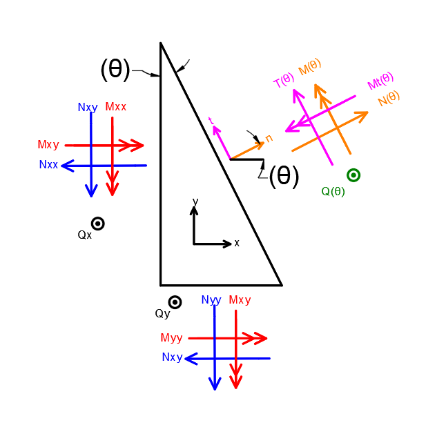
Figure 16. **Corner balance and transition from « 2D » to « 1D » efforts

We find:

\(N\left(\theta \right)={N}_{\mathit{xx}}\times \mathit{co}{s}^{2}\left(\theta \right)+2\times {N}_{\mathit{xy}}\times \mathrm{cos}\left(\theta \right)\times \mathrm{sin}\left(\theta \right)+{N}_{\mathit{yy}}\times \mathit{si}{n}^{2}\left(\theta \right)\)

\(M\left(\theta \right)={M}_{\mathit{xx}}\times \mathit{co}{s}^{2}\left(\theta \right)+2\times {M}_{\mathit{xy}}\times \mathrm{cos}\left(\theta \right)\times \mathrm{sin}\left(\theta \right)+{M}_{\mathit{yy}}\times \mathit{si}{n}^{2}\left(\theta \right)\)

\(T\left(\theta \right)=\frac{-1}{2}\times {N}_{\mathit{xx}}\times \mathrm{sin}\left(2\theta \right)+{N}_{\mathit{xy}}\times \mathrm{cos}\left(2\theta \right)+\frac{1}{2}\times {N}_{\mathit{yy}}\times \mathrm{sin}\left(2\theta \right)\)

\({M}_{t}\left(\theta \right)=\frac{-1}{2}\times {M}_{\mathit{xx}}\times \mathrm{sin}\left(2\theta \right)+{M}_{\mathit{xy}}\times \mathrm{cos}\left(2\theta \right)+\frac{1}{2}\times {M}_{\mathit{yy}}\times \mathrm{sin}\left(2\theta \right)\)

\(Q\left(\theta \right)=-{Q}_{x}\times \mathrm{cos}\left(\theta \right)-{Q}_{y}\times \mathrm{sin}\left(\theta \right)\)

Such as:

\(N\left(\theta \right)\mathit{et}M\left(\theta \right)\) Use the fictional beam in Compound Flexion (FC)
\(T\left(\theta \right)\mathit{et}{M}_{t}\left(\theta \right)\) Use the fictional girder in Membrane Shear (CISA)
\(Q\left(\theta \right)\) Request the fictional beam in Off-Plane Shear (CISHP)

As used in its current version, the “classical” Capra Maury method would only cover the verification of the normal effort \(N\left(\theta \right)\) and the bending moment \(M\left(\theta \right)\) as membrane forces, the stresses \(T\left(\theta \right)\mathit{et}{M}_{t}\left(\theta \right)\) being neglected.

In this sense, for \(\theta\) ranging from 0 to 360°, we would be reduced to the sizing of a fictional composite bending beam, such as determining the upper \({A}_{s,s}\left(\theta \right)\) and lower \({A}_{s,i}\left(\theta \right)\) steel sections required for balance, in accordance with the principles of dimensioning beams as explained in paragraph 1 of the documentation.

This reinforcement is « fictional » and it is felt by the projection of the reinforcement beds actually arranged in the plate, namely the projection of the steel sections along the x and y axes respectively, and along the upper and lower face of the slab.

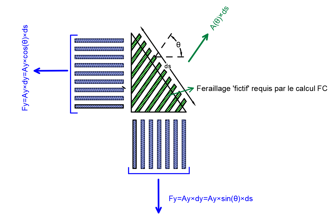
Figure 17.Projection of the reinforcement beds and Composition of the fictional reinforcement by facet considered

Thus, by referring to the “real” reinforcement of the slab/wall, namely quadruplet \(({A}_{\mathit{sx},s},{A}_{\mathit{sy},s},{A}_{\mathit{sx},i},{A}_{\mathit{sy},i}\text{}\mathit{en}{\mathit{cm}}^{2}/\mathit{ml}),\), it will be necessary to verify, in accordance with the previous figure, the two inequalities below:

For the upper side: \({A}_{\mathit{sx},s}\times {\mathrm{cos}}^{2}\mathrm{\theta }+{A}_{\mathit{sy},s}\times {\mathrm{sin}}^{2}\mathrm{\theta }⩾{A}_{s,s}(\mathrm{\theta })\)

For the underside: \({A}_{\mathit{sx},i}\times {\mathrm{cos}}^{2}\mathrm{\theta }+{A}_{\mathit{sy},i}\times {\mathrm{sin}}^{2}\mathrm{\theta }⩾{A}_{s,i}(\mathrm{\theta })\)

In what follows, we limit ourselves to only one side of the section (lower or upper), such as we seek to minimize the sum (\(({A}_{\mathit{sx}}+{A}_{\mathit{sy}})\)) while verifying that the two terms obviously remain positive. To do this, we use graphical reasoning and we draw the equation line in the orthonormal coordinate system (Asx, Asy), for each angle θ considered:

\(\left({d}_{\theta }\right)\mathrm{:}{A}_{\mathit{sy}}=\frac{{A}_{s}(\theta )}{{\mathrm{sin}}^{2}(\theta )}-{A}_{\mathit{sx}}\times {\mathit{cotn}}^{2}(\theta )\)

The set of lines thus drawn would delimit a validation domain constructed through the intersections of these lines, and guaranteeing the respect of the inequalities given previously for each value of θ considered — note of course, that we would have two distinct sets of lines: one for the equilibrium in the upper table and another for the balance in the lower table.

Knowing that for a given line, its domain of validity is the part of the coordinate system located above the line, all the lines drawn would therefore constitute a convex polygon « open » upward, whose vertices are none other than the intersections of the various lines (dθ). These last points are therefore reinforcing pairs (Ax; Ay) i solutions to the overall balance of the upper/lower sheet. In particular, in view of the convexity of the constructed validation domain, these points would lead to the minimum reinforcement (that is to say to the solutions giving the smallest amounts (Ax+Ay)) of the entire field of validity, and finally the point allowing to minimize the distance “d” between its orthogonal projection on the 1st bisector of the plane and the origin of the coordinate system (cf. in the figure below) will be retained.).

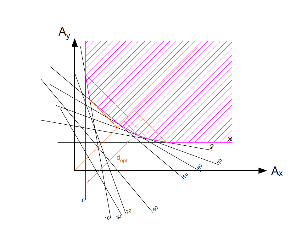
Figure 18. Construction of the validation domain by table (Sup and Inf)

Concretely, in the algorithm, we define a discrete set of facets centered at the point of calculation, whose normal rotates in the tangential plane to the middle sheet. The angle \(\mathrm{\theta }\) of the facets is discretized regularly from \(-90°\) to \(+90°\), taking into account the symmetry of the equilibrium inequalities.

2.1.2. Consideration of Off-Plane Shear#

This part involves the resumption of the transverse shear forces of the facets, namely \(Q\left(\theta \right)\) with:

\(Q\left(\theta \right)=-{Q}_{x}\times \mathrm{cos}\left(\theta \right)-{Q}_{y}\times \mathrm{sin}\left(\theta \right)\)

The use of \(Q\left(\theta \right)\) by each of the “fictional girders” corresponds to a classical study of the transverse shear force of a beam (§6.2 of EN-1992-1).

According to the clauses and formulas developed in this paragraph of Eurocode 2, a transverse reinforcement \({A}_{\mathit{sv},\mathit{CISHP}}(\theta )\) (in the case where \(Q\left(\theta \right)>{V}_{\mathit{Rd},c,z}(\theta )\)) will be calculated, considering:

Beam height: \(h=e\), “e” being the thickness of the plate
Width of the beam: \(b=1m\)
Useful height for calculation: \(d=\{\begin{array}{c}h-{c}_{\text{inf}}\mathit{si}M\left(\theta \right)>0\\ h-{c}_{\text{sup}}\mathit{si}M\left(\theta \right)<0\end{array}\)
Calculation lever arm: \(z=\left[\left[{A}_{s,\mathit{comp}}\times {\sigma }_{\mathit{As},\mathit{comp}}\right]\times {z}_{1}+\left[{F}_{\mathit{cc}}\right]\times {z}_{2}\right]/\left[{A}_{s,\mathit{comp}}\times {\sigma }_{\mathit{As},\mathit{comp}}+{F}_{\mathit{cc}}\right]\)

Where

\({A}_{s,\mathit{comp}}\): refers to the compressed steel section (if required by the Compound Flexion calculation)
\({\sigma }_{\mathit{As},\mathit{comp}}\): refers to the stress felt at the right of compressed steel (as given by the FC calculation and according to the associated deformation diagram)
\({z}_{1}=\{\begin{array}{c}d-{c}_{\text{sup}}\mathit{si}M\left(\theta \right)>0\\ d-{c}_{\text{inf}}\mathit{si}M\left(\theta \right)<0\end{array}\): refers to the lever arm of the compression steel in relation to the center of gravity of the tensile steel (main reinforcement)
\({F}_{\mathit{cc}}\): refers to the total force taken up by the compressed concrete (as given by the FC calculation and according to the associated deformation diagram)
\({z}_{2}\): refers to the lever arm of the \({F}_{\mathit{cc}}\) force in relation to the center of gravity of the traction steel (main reinforcement)

Figure 19 .Calculation of transverse reinforcement for the recovery of Off-plane Shear (CISHP)

From here, we refer to the “real” transverse reinforcement of the slab/wall (i.e. the reinforcing pair \(\left({A}_{\mathit{sv}}{,}_{x};{A}_{\mathit{sv}}{,}_{y}\right)\) expressed in cm2/m/m).

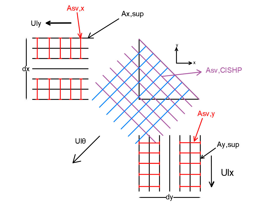
Figure 20. **Global balance and calculation of out-of-plane shear reinforcement

Thus, following a reasoning similar to that adopted for the determination of membrane reinforcement, it will be a question of verifying the inequality below for each facet orientation considered:

\({A}_{\mathit{sv},x}\times {\mathrm{cos}}^{2}\theta +{A}_{\mathit{sv},y}\times {\mathrm{sin}}^{2}\theta \ge {A}_{\mathit{sv}}{,}_{\mathit{CISHP}}(\theta )\)

The resolution is carried out graphically, in the same way as the explanations explained in §2.1.1.

2.2. Sandwich method#

2.2.1. Principle of the method#

The Sandwich method — initiated in the literature by Gupta and Marti and whose principle was introduced (but in an incomplete and not very detailed way) in Annex LL of EN-1992-2 in 2004 — is a method that makes it possible to value the 2D character of a plate element, taking into account the bi-directional stiffness of the element as well as the plate kinematics (the latter point being supported by the additional step of the escalation that will be introduced later in the note).

This method divides the plate into 3 layers (hence the name):

The upper and lower layers (with respective thicknesses**tsup**and**tinf*) resist membrane stresses (normal forces, bending moment, membrane shear and twisting). They therefore resume the \({N}_{\mathit{xx}},{N}_{\mathit{yy}}\mathit{et}{N}_{\mathit{xy}}\) efforts as well as the \({M}_{\mathit{xx}},{M}_{\mathit{yy}}\mathit{et}{M}_{\mathit{xy}}\) efforts.

The intermediate layer or concrete core (**tc* thick) resists out-of-plane shear. So she is resuming the \({Q}_{x}\mathit{et}{Q}_{y}\) efforts.

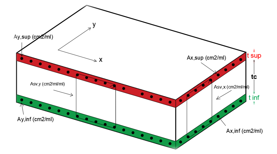
Figure 21.Presentation of the « Sandwich » model (division of the plate into 3 layers)

Thus, the first step of the method is to determine, by means of an iterative calculation, the optimal thicknesses of the two peripheral layers and then to deduce the membrane reinforcement (i.e. the quadruplet (\({A}_{\text{x,sup}},{A}_{\text{y,sup}},{A}_{\text{x,inf}},{A}_{\text{y,inf}}\)) in cm2/ml). In a second step, the thickness of the intermediate layer can be deduced (tc = h—tsup—tinf) and the transverse reinforcement (i.e. the pair (\({A}_{\mathit{sv},x},{A}_{\mathit{sv},y}\)) in cm2/ml/ml) will be calculated according to the classical rules for the shear force design of beams as developed in §6.2 of EN-1992-1.

2.2.2. Determination of membrane balance#

We start by calculating the “felt” forces at the centers of gravity of the upper (SUP) and lower (INF) reinforcement layers.

Thus, in accordance with the following notations, we will have:

For the top table:

\({N}_{\text{xx,sup}}={N}_{\mathit{xx}}\times \left(\frac{z-{y}_{\text{sup}}}{z}\right)+\frac{{M}_{\mathit{xx}}}{z}+\frac{1}{2}\times {D}_{\mathit{nxx}}\)

\({N}_{\text{yy,sup}}={N}_{\mathit{yy}}\times \left(\frac{z-{y}_{\text{sup}}}{z}\right)+\frac{{M}_{\mathit{yy}}}{z}+\frac{1}{2}\times {D}_{\mathit{nyy}}\)

\({N}_{\text{xy,sup}}={N}_{\mathit{xy}}\times \left(\frac{z-{y}_{\text{sup}}}{z}\right)+\frac{{M}_{\mathit{xy}}}{z}+\frac{1}{2}\times {D}_{\mathit{nxy}}\)

For the lower table:

\({N}_{\mathit{xx},\mathit{inf}}={N}_{\mathit{xx}}\times \left(\frac{z-{y}_{\mathit{inf}}}{z}\right)-\frac{{M}_{\mathit{xx}}}{z}+\frac{1}{2}\times {D}_{\mathit{nxx}}\)

\({N}_{\mathit{yy},\mathit{inf}}={N}_{\mathit{yy}}\times \left(\frac{z-{y}_{\mathit{inf}}}{z}\right)-\frac{{M}_{\mathit{yy}}}{z}+\frac{1}{2}\times {D}_{\mathit{nyy}}\)

\({N}_{\mathit{xy},\mathit{inf}}={N}_{\mathit{xy}}\times \left(\frac{z-{y}_{\mathit{inf}}}{z}\right)-\frac{{M}_{\mathit{xy}}}{z}+\frac{1}{2}\times {D}_{\mathit{nxy}}\)

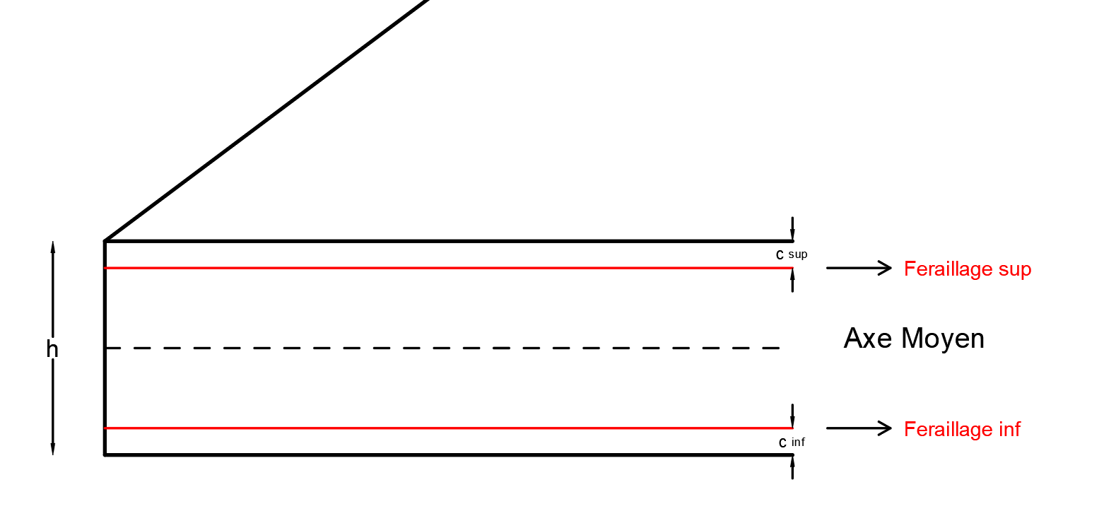
Figure 22.Distribution of membrane forces between layers SUP and INF

As we know:

Eccentricity of the tablecloth SUP: \({y}_{\text{sup}}=h/2-{c}_{\text{sup}}\)
Eccentricity of the tablecloth INF: \({y}_{\mathit{inf}}=h/2-{c}_{\mathit{inf}}\)
Internal force lever arm: \(z={y}_{\text{sup}}+{y}_{\mathit{inf}}\)

The**Dnxx*,**Dnyy**and**Dnxy** forces are the tensile forces due to the Ritter-Morsch mesh for the resumption of transverse shear in the intermediate layer (at the beginning of the algorithm, these forces are zero, then we will iterate).

The condition of each steel sheet is then evaluated (the reasoning for sheet SUP is given as an indication):

if:Math: {N} _ {text {xx, sup}}ge -left| {N} _ {text {xy, sup}}right| and:math:` {N} _ {text {n} _ {text {xx, sup} _ {text {xy, sup}} _ {text {xy, sup}}right|`, then CAS_SUP = 1
Otherwise, if:math: {N} _ {text {xx, sup}} {text {xx, sup}} <-left| {N} _ {text {xy, sup}}right| et:math:` {N} _ {text {yy, sup}} > {text {xy, sup}}} ^ {2}/{N} _ {text {xx, sup}} _ {text {xx, sup}}} `, then CAS_SUP = 2
Otherwise, if:math: {N} _ {text {xx, sup}} {text {xx, sup}}} <-left| {N}}right| and:math:` {N} _ {text {N} _ {text {yy, sup} _ {text {yy, sup}}} <-text {xx, sup}}} <-text {xx, sup}}}le {N} _ {text {xx, sup}} {text {xy, sup}} ^ {2}/{N} _ {text {N}} _ {text {xx, sup}} _ {text {xx, sup}}} `, then CAS_SUP = 3
Otherwise, if:math: {N} _ {text {yy, sup} _ {text {yy, sup}} <-left| {N} _ {text {xy, sup}}right| et:math:` {N} _ {text {xx, sup}} > {text {xy, sup}}} ^ {2}/{N} _ {text {yy, sup}} _ {text {yy, sup}}} `, then CAS_SUP = 3
Otherwise, if:math: {N} _ {text {yy, sup}}} <-left| {N} _ {text {xy, sup}}right| and:math:` {N} _ {text {N} _ {text {xx, sup} _ {text {xx, sup}}}le {x, sup}} _ {text {xy, sup}} ^ {2}/{N} _ {text {N}} _ {text {y, sup} _ {text {yy, sup}} _ {text {yy, sup}} _ {text {yy, sup}}} `, then CAS_SUP = 4
If not, then CAS_SUP = 4

In this sense, we will have the following cases:

CAS_SUP = 1 traction reinforcement required in the x and y directions of the SUP sheet
CAS_SUP = 2 traction reinforcements required in the y direction only of the SUP sheet
CAS_SUP = 3 traction reinforcements required in the x-direction only of the SUP sheet
CAS_SUP = 4 steps of traction reinforcement required for the SUP sheet

From there, according to the values taken by CAS_SUP and by CAS_INF, the algorithm of the method is structured according to 4 main components as supported below:

If CAS_SUP > 4 and CAS_INF > 4 CAS_SAND = 1
Otherwise, if CAS_SUP .pl 4 and CAS_INF = 4 CAS_SAND = 2
Otherwise, if CAS_SUP = 4 and CAS_INF 497 = 4 CAS_SAND = 3
Otherwise CAS_SAND = 4

Such as:

CAS_SAND = 1 traction reinforcement required in layers SUP and INF
**** CAS_SAND =****2** tensile reinforcement required in sheet SUP only (the tinf layer being governed by a state of bi-axial compression)
**** CAS_SAND =****3** tensile reinforcement required in sheet INF only (the tsup layer being governed by a state of bi-axial compression)
CAS_SAND = 4 no traction reinforcement required (fully compressed plate)

The idea is then to write the membrane balance according to the case in question and to determine the thicknesses of the two layers SUP and INF, as well as the main membrane reinforcement of the plate.

2.2.2.1. 1st configuration: CAS_SAND = 1#

In this first case considered, each peripheral layer (SUP and INF) will be characterized by:

Its thickness (tsup/inf)
Two resisting “positive” (tensile) steel forces (following x: nsx and following y: nsy)
A resisting “negative” (compression) force taken up by a compression rod (nc) whose direction is to be determined (angle θ formed with the « y » axis); in fact, the tensile reinforcement being required, there would be at least one main tensile stress at the level of each layer (and therefore at most, a single compression rod per layer).

The global membrane equilibrium equations are then written as follows:

\({N}_{\text{xx}}={n}_{\text{sx,sup}}+{n}_{\text{sx,inf}}+{n}_{\text{c,sup}}\times {\mathrm{sin}}^{2}\left({\theta }_{\text{sup}}\right)+{n}_{\text{c,inf}}\times {\mathrm{sin}}^{2}\left({\theta }_{\text{inf}}\right)[E1]\)

\({N}_{\text{yy}}={n}_{\text{sy,sup}}+{n}_{\text{sx,inf}}+{n}_{\text{c,sup}}\times {\mathrm{cos}}^{2}\left({\theta }_{\text{sup}}\right)+{n}_{\text{c,inf}}\times {\mathrm{cos}}^{2}\left({\theta }_{\text{inf}}\right)\text{}[E2]\)

\({N}_{\mathit{xy}}={n}_{\text{c,sup}}\times \mathrm{cos}\left({\theta }_{\text{sup}}\right)\times \mathrm{sin}({\theta }_{\text{sup}})+{n}_{\text{c,inf}}\times \mathrm{cos}\left({\theta }_{\text{inf}}\right)\times \mathrm{sin}\left({\theta }_{\text{inf}}\right)\text{}[E3]\)

\({M}_{\text{xx}}={n}_{\text{sx,sup}}\times {y}_{\text{sup}}-{n}_{\text{sx,inf}}\times {y}_{\text{inf}}+{m}_{\text{c,sup}}\times {\mathrm{sin}}^{2}\left({\theta }_{\text{sup}}\right)-{m}_{\text{c,inf}}\times {\mathrm{sin}}^{2}\left({\theta }_{\text{inf}}\right)\text{}[E4]\)

\({M}_{\text{yy}}={n}_{\text{sy,sup}}\times {y}_{\text{sup}}-{n}_{\text{sy,inf}}\times {y}_{\text{inf}}+{m}_{\text{c,sup}}\times {\mathrm{cos}}^{2}\left({\theta }_{\text{sup}}\right)-{m}_{\text{c,inf}}\times {\mathrm{cos}}^{2}\left({\theta }_{\text{inf}}\right)\text{}[E5]\)

\({M}_{\text{xy}}={m}_{\text{c,sup}}\times \mathrm{cos}\left({\theta }_{\text{sup}}\right)\times \mathrm{sin}({\theta }_{\text{sup}})-{m}_{\text{c,inf}}\times \mathrm{cos}\left({\theta }_{\text{inf}}\right)\times \mathrm{cos}\left({\theta }_{\text{inf}}\right)\text{}[E6]\)

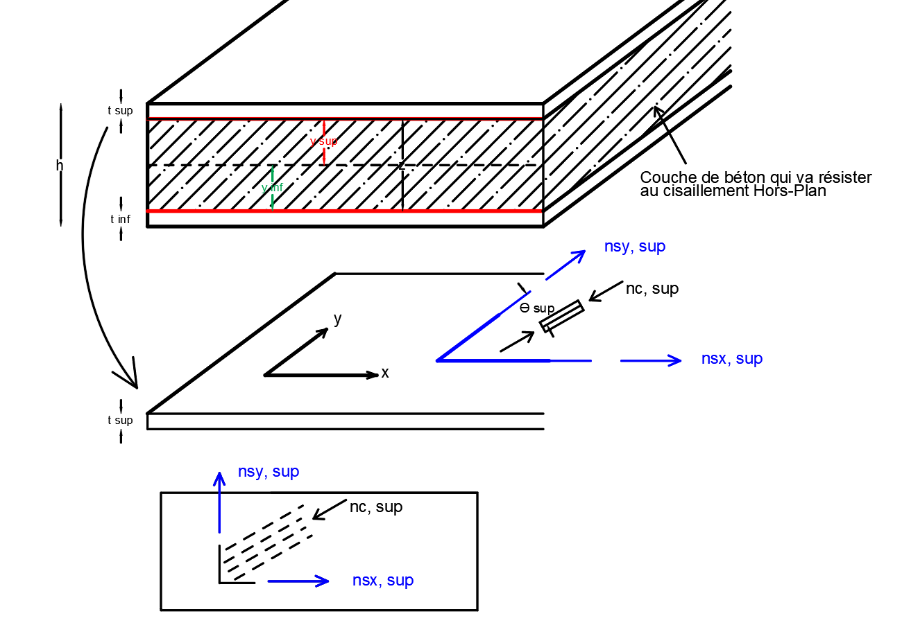
Figure 23.Slab configuration (steel forces and orientation of concrete rods)

In this first case, we would thus have:

6 equations for 8 unknowns: θ sup; θ inf; θ inf; tsup; Asx, sup; Asy, sup; Asx, inf; Asx, inf; Asy, inf

Such as:

nsx, sup=Asx, supfyd; nsy, supfyd; nsy, supfyd; nsx, inf=Asx, inffyd; nsy, inf=Asy, inffyd; nsy, inf=Asy, inffyd

nc, sup = -tsupfc, sup; nc, nc, inf = -tinffc, inf = -tinffc, inf; mc, inf = 0.5 x (h — tinf) x (h — tsup) x nc, inf; mc, mc, inf = 0.5 x (h — tinf) x nc, inf

In particular, the strength of the compression rods is determined in accordance with the provisions of §6.109 - Membrane elements of EN-1992-2 (Case of a “partially compressed” plate):

\({f}_{\text{c,sup/inf}}={f}_{\mathit{cd}1}={f}_{\mathit{cd}}\times \left[0.85-\frac{{\sigma }_{s}}{{f}_{\mathit{yd}}}\times (0.85-\vartheta )\right]\)

Or:

:math:`{sigma }_{s}` represents the stress experienced in steel (we’ll take :math:`{sigma }_{s}={f}_{mathit{yd}}`)

\(\vartheta =0.6\times \left[1-{f}_{\mathit{ck}}/250\right]\).

**NOTA:* for the moment, it is considered that the reinforcements and the compression rods are working simultaneously at their ultimate limit states. In reality, it will be necessary to incorporate into the problem the search for the deformation field (in a manner similar to the rule of 3 pivots for composite bending beams) from which we will deduce, according to the laws of material behavior, the material (compressed concrete or tension steel) that works at its ultimate limit state and therefore dictating the shape of the deformation diagram and therefore the stresses actually felt.

2.2.2.2. 2nd configuration: CAS_SAND = 2#

In this case, only layer SUP requires positive tensile reinforcement; layer INF being governed by a bi-axial compression field, no reinforcement is required (for this reason, for the moment, it is assumed that the compressive stresses remain relatively low compared to the ultimate capacity of concrete, and that consequently a “negative” compression reinforcement is not envisaged). So:

Layer SUP will always be characterized by its thickness**tsup*, the inclination of its compression rod**θ sup**and the resistive force that it takes up (nc, sup**= -tsup x fc, sup), as well as the reinforcement forces**nsx, sup, and**nsy, sup**, positive (traction).

Layer INF will be characterized by its**tinf* thickness, and by the field of stresses affecting the concrete included in the coordinate system (x, y), namely:

\(\left(\begin{array}{c}{n}_{\mathit{cx},\mathit{inf}}\\ {n}_{\mathit{cxy},\mathit{inf}}\end{array}\begin{array}{c}{n}_{\mathit{cxy},\mathit{inf}}\\ {n}_{\mathit{cy},\mathit{inf}}\end{array}\right)\)

These efforts are negative since it is a state of compression, the coordinate system (x, y) not necessarily being the main frame of reference of the stress field in layer INF (it will be so if and only if \({n}_{\mathit{cxy},\mathit{inf}}=0\)). The main constraints can be deduced by diagonalizing the matrix.

The membrane balance of the system is now written as follows:

\({N}_{\text{xx}}={n}_{\text{sx,sup}}+{n}_{\text{c,sup}}\times {\mathrm{sin}}^{2}\left({\theta }_{\text{sup}}\right)+{n}_{\text{cx,inf}}\text{}[E1]\)

\({N}_{\text{yy}}={n}_{\text{sy,sup}}+{n}_{\text{c,sup}}\times {\mathrm{cos}}^{2}\left({\theta }_{\text{sup}}\right)+{n}_{\mathit{cy},\mathit{inf}}\text{}[E2]\)

\({N}_{\text{xy}}={n}_{\text{c,sup}}\times \mathrm{cos}\left({\theta }_{\text{sup}}\right)\times \mathrm{sin}({\theta }_{\text{sup}})+{n}_{\text{cxy,inf}}\text{}[E3]\)

\({M}_{\text{xx}}={n}_{\text{sx,sup}}\times {y}_{\text{sup}}+{m}_{\text{c,sup}}\times {\mathrm{sin}}^{2}\left({\theta }_{\text{sup}}\right)-{m}_{\text{cx,inf}}\text{}[E4]\)

\({M}_{\text{yy}}={n}_{\text{sy,sup}}\times {y}_{\text{sup}}+{m}_{\text{c,sup}}\times {\mathrm{cos}}^{2}\left({\theta }_{\text{sup}}\right)-{m}_{\text{cy,inf}}\text{}[E5]\)

\({M}_{\text{xy}}={m}_{\text{c,sup}}\times \mathrm{cos}\left({\theta }_{\text{sup}}\right)\times \mathrm{sin}({\theta }_{\text{sup}})-{m}_{\mathit{cxy},\mathit{inf}}\text{}[E6]\)

Such as:

nsx, sup=Asx, supfyd; nsy, sup=Asy, supfyd; nsy, supfyd

nc, sup = -tsupfc, sup; mc, mc, sup = 0.5 x (h — tsup) x nc, sup

mcx, inf = 0.5 x (h — tinf) x ncx, inf; mcy, inf = 0.5 x (h — tinf) x ncy, inf; mcxy, inf = 0.5 x (h — tinf) x ncxy, inf

In addition, in accordance with the preceding explanations, by diagonalizing the force matrix in layer INF, the main major compression force is obtained below:

\({n}_{c,\mathit{inf}}={-t}_{\mathit{inf}}\times {f}_{c,\mathit{inf}}=\frac{1}{2}\times \left({n}_{\mathit{cx},\mathit{inf}}+{n}_{\mathit{cy},\mathit{inf}}\right)-\sqrt{{\left(\frac{{n}_{\mathit{cx},\mathit{inf}}+{n}_{\mathit{cy},\mathit{inf}}}{2}\right)}^{2}+{n}_{\mathit{cxy},\mathit{inf}}^{2}}\text{}[E7]\)

And now we would have:

7 equations for 8 unknowns: †sup; tsup; tsup; tinf; Asx, sup; ncx, inf; ncx, inf; ncy, inf;**ncy, inf; ****ncy, inf; ****ncxy, inf

In particular, the strength of compression rods is determined in accordance with the provisions of §6.109 - Membrane elements of EN-1992-2:

\({f}_{\text{c,sup}}={f}_{\mathit{cd}1}={f}_{\mathit{cd}}\times \left[0.85-\frac{{\sigma }_{s}}{{f}_{\mathit{yd}}}\times (0.85-\vartheta )\right]\) (Case of a “partially compressed” plaque)

\({f}_{c,\mathit{inf}}={f}_{\mathit{cd}2}=0.85\times {f}_{\mathit{cd}}\times \frac{1+3.8{\alpha }_{\mathit{inf}}}{{\left(1+{\alpha }_{\mathit{inf}}\right)}^{2}}\) (Case of a “fully compressed” plate)

For example, αinf refers to the ratio of the main compression stresses in layer INF:

math:: {alpha} _ {mathit {cx}} | {mathit {inf}}} =left|frac {1} {2}timesleft ({n} _ {mathit {cx}},mathit {cx}},mathit {cx},mathit {cx},mathit {cx},mathit {cx},mathit {cx},mathit {cx},mathit {cx}},mathit {cx},mathit {cx},mathit {cx},mathit {cx},mathit {cx},mathit {cx},mathit {cx},mathit {cx},mathit {cx},mathit {cx},mathit {{n} _ {mathit {cx},mathit {cx},mathit {inf}}} + {n}} _ {mathit {cy}}} {2}right)} ^ {2} + {n} + {n} _ {n} _ {mathit {inf}}} {mathit {cxy}},mathit {cxy}},mathit {cxy}},mathit {cxy},mathit {cxy},mathit {cxy},mathit {cxy},mathit {inf}}}} {frac {1} {2} {2}}timesleft (n {} _ {mathit {cx},mathit {cx}} + {n}} + {n} _ {mathit {cy},mathit {inf}}right) -sqrt {{left (frac {{n}} _ {frac {n}} _ {frac {n}} _ {frac {{n}} _ {left (frac {{n}} _ {frac {n}} _ {frac {n}} _ {frac {n}} _ {frac {{n}} _ {frac {n}} _ {frac {n}} _ {frac {n}} _ {frac {n}} _ {frac {n}} _ {frac {}right)} ^ {2} + {n} _ {mathit {cxy},mathit {inf}} ^ {2}}}}right|le 1

2.2.2.3. 3rd configuration: CAS_SAND = 3#

This case is symmetric to the previous case.

In this case, only layer INF requires positive tensile reinforcement; layer SUP being governed by a bi-axial compression field, no reinforcement is required.

2.2.2.4. 4th configuration: CAS_SAND = 4#

In this case, no layer requires positive tensile reinforcement; the two layers SUP and INF being governed by bi-axial compression fields. The membrane balance equations are then written as follows:

\({N}_{\text{xx}}={n}_{\text{cx,inf}}+{n}_{\text{cx,sup}}\text{}[E1]\)

\({N}_{\text{yy}}={n}_{\text{cy,inf}}+{n}_{\text{cy,sup}}\text{}[E2]\)

\({N}_{\text{xy}}={n}_{\text{cxy,inf}}+{n}_{\text{cxy,sup}}\text{}[E3]\)

\({M}_{\text{xx}}={m}_{\text{cx,sup}}-{m}_{\text{cx,sinf}}\text{}[E4]\)

\({M}_{\text{yy}}={m}_{\text{cy,sup}}-{m}_{\text{cy,sinf}}\text{}[E5]\)

\({M}_{\text{xy}}={m}_{\text{cxy,sup}}-{m}_{\text{cxy,sinf}}\text{}[E6]\)

Such as:

mcx, sup = 0.5 x (h — tsup) x ncx, sup; mcy, sup = 0.5 x (h — tsup) x ncy, sup; mcxy, sup = 0.5 x (h — tsup) x ncxy, sup = 0.5 x (h — tsup) x ncxy, sup

mcx, inf = 0.5 x (h — tinf) x ncx, inf; mcy, inf = 0.5 x (h — tinf) x ncy, inf; mcxy, inf = 0.5 x (h — tinf) x ncxy, inf

Moreover, by diagonalizing the force matrices in layers SUP and INF, the respective main major compression forces are obtained below:

\({n}_{\text{c,sup}}={-t}_{\text{sup}}\times {f}_{\text{c,sup}}=\frac{1}{2}\times \left({n}_{\text{cx,sup}}+{n}_{\text{cy,sup}}\right)-\sqrt{{\left(\frac{{n}_{\text{cx,sup}}+{n}_{\text{cy,sup}}}{2}\right)}^{2}+{n}_{\text{cxy,sup}}^{2}}\text{}[E7]\)

And now we would have:

8 equations for 8 unknowns: tsup; tinf; ncx, sup; ncy, sup; ncxy, sup; ncx, inf; ncy, inf; ncy, inf;**ncy, inf; ****ncxy, inf

In particular, the strength of compression rods is determined in accordance with the provisions of §6.109 - Membrane elements of EN-1992-2:

\({f}_{\text{c,sup}}={f}_{\mathit{cd}2}=0.85\times {f}_{\mathit{cd}}\times \frac{1+3.8{\alpha }_{\text{sup}}}{{\left(1+{\alpha }_{\text{sup}}\right)}^{2}}\) (Case of a “fully compressed” plate)

2.2.2.5. Consideration of “negative” compression reinforcement#

From a numerical point of view, such a case occurs when, with the macros introduced previously (CAS_SAND = 1, 2, 3 or 4), one obtains one of the following scenarios:

If in the loop CAS_SAND = 1 (tension reinforcement required in SUP and INF), we have one of the calculated terms \({n}_{\text{sx,sup}},{n}_{\text{sy,sup}},{n}_{\text{sx,inf}},{n}_{\text{sy,inf}}\) which is negative, then we do not change anything in this case since the equilibrium equations are always the same The forces at negative values indicate that it is a compression reinforcement according to the sheet and the direction considered.

Likewise, if in the loop CAS_SAND = 2 (tensile reinforcement required in SUP), the algorithm results in a solution of the problem with at most one of the negative steel forces in SUP Nothing to change, the forces with negative values indicate that it is a compression reinforcement according to the sheet and the direction considered. However, if the balance cannot be achieved (i.e. inability to determine the unknowns of the problem, including in particular the thicknesses of the two layers SUP and INF), a new scenario is then introduced which will be designated* CAS_SAND =**=** 2bis.

Same observation for the CAS_SAND = 3 loop (and possible introduction of the scenario* CAS_SAND = 3 bis**).

If in the loop CAS_SAND = 4 the balance cannot be achieved (i.e. inability to determine the unknowns of the problem, including in particular the thicknesses of the two layers SUP and INF), a new scenario is then introduced that will be designated* CAS_SAND =****4bis**.

In what follows, the analytical approach of the three additional cases developed to cover compression reinforcement appropriately, and appropriately to the case from which it derives, is therefore presented.

CAS_SAND = 2 bis « « » « « » « » « « » »

In this new case, we would now have simultaneously, in layer INF:

*2 steel beds according to x and y, using the forces \({n}_{\mathit{sx},\mathit{inf}}\) and \({n}_{\mathit{sy},\mathit{inf}}\) respectively (the calculation should give*negative values to these forces, in the case of compression reinforcements).

2 main compression rods, namely \({n}_{c,\mathit{inf},\mathit{max}}\) and \({n}_{c,\mathit{inf},\mathit{min}}\) (these efforts are also negative). In order to simplify the process and simplify the notations, we will consider as unknown to the problem, the maximum constraint by setting \({n}_{c,\mathit{inf}}={n}_{c,\mathit{inf},\mathit{max}}\) and its orientation in the coordinate system (x, y) given by the angle \({\theta }_{\mathit{inf}}\) that its direction makes with the y axis (the orientation of \({n}_{c,\mathit{inf},\mathit{min}}\) being given by \(\pi /2+{\theta }_{\mathit{inf}}\)), as well as the ratio of the two main constraints, namely \({\alpha }_{\mathit{inf}}={n}_{c,\mathit{inf},\mathit{min}}/{n}_{c,\mathit{inf},\mathit{max}}\).

In this new case, writing the membrane balance equations then leads to:

\({N}_{\mathit{xx}}={n}_{\text{sx,sup}}+{n}_{\text{sx,inf}}+{n}_{\text{c,sup}}\times {\mathrm{sin}}^{2}\left({\theta }_{\text{sup}}\right)+{n}_{\text{c,inf}}\times \left[{\mathrm{sin}}^{2}\left({\theta }_{\text{inf}}\right)+{\alpha }_{\text{inf}}\times {\mathrm{cos}}^{2}({\theta }_{\text{inf}})\right]\text{}[E1]\)

\({N}_{\mathit{yy}}={n}_{\text{sy,sup}}+{n}_{\text{sy,inf}}+{n}_{\text{c,sup}}\times {\mathrm{cos}}^{2}\left({\theta }_{\text{sup}}\right)+{n}_{\text{c,inf}}\times \left[{\mathrm{cos}}^{2}\left({\theta }_{\text{inf}}\right)+{\alpha }_{\text{inf}}\times {\mathrm{sin}}^{2}({\theta }_{\text{inf}})\right]\text{}[E2]\)

\({N}_{\mathit{xy}}={n}_{\text{c,sup}}\times \mathrm{cos}\left({\theta }_{\text{sup}}\right)\times \mathrm{sin}({\theta }_{\text{sup}})+{(1-{\alpha }_{\text{inf}})\times n}_{\text{c,inf}}\times \mathrm{cos}\left({\theta }_{\text{inf}}\right)\times \mathrm{sin}\left({\theta }_{\text{inf}}\right)\text{}[E3]\)

\({M}_{\mathit{xx}}={n}_{\text{sx,sup}}\times {y}_{\text{sup}}-{n}_{\text{sx,inf}}\times {y}_{\text{inf}}+{m}_{\text{c,sup}}\times {\mathrm{sin}}^{2}\left({\theta }_{\text{sup}}\right)-{m}_{\text{c,inf}}\times \left[{\mathrm{sin}}^{2}\left({\theta }_{\text{inf}}\right)+{\alpha }_{\text{inf}}\times {\mathrm{cos}}^{2}\left({\theta }_{\text{inf}}\right)\right]\text{}[E4]\)

\({M}_{\mathit{yy}}={n}_{\text{sy,sup}}\times {y}_{\text{sup}}-{n}_{\text{sy,inf}}\times {y}_{\text{inf}}+{m}_{\text{c,sup}}\times {\mathrm{cos}}^{2}\left({\theta }_{\text{sup}}\right)-{m}_{\text{c,inf}}\times \left[{\mathrm{cos}}^{2}\left({\theta }_{\text{inf}}\right)+{\alpha }_{\text{inf}}\times {\mathrm{sin}}^{2}\left({\theta }_{\text{inf}}\right)\right]\text{}[E5]\)

\({M}_{\mathit{xy}}={m}_{\text{c,sup}}\times \mathrm{cos}\left({\theta }_{\text{sup}}\right)\times \mathrm{sin}({\theta }_{\text{sup}})-{\left(1-{\alpha }_{\text{inf}}\right)\times m}_{\text{c,inf}}\times \mathrm{cos}\left({\theta }_{\text{inf}}\right)\times \mathrm{sin}\left({\theta }_{\text{inf}}\right)\text{}[E6]\)

In addition, taking into account the provisions of §6.109 of EN-1992-2, we would also have the following relationships:

\({n}_{\text{c,sup}}={-t}_{\text{sup}}\times {f}_{\text{c,sup}}={-t}_{\text{sup}}\times {f}_{\text{cd1}}\) (Case of a “partially compressed” plaque)

\({n}_{c,\mathit{inf}}={-t}_{\mathit{inf}}\times {f}_{c,\mathit{inf}}={-t}_{\mathit{inf}}\times {f}_{\mathit{cd}2}={-t}_{\mathit{inf}}\times 0.85\times {f}_{\mathit{cd}}\times \frac{\left(1+3.8\times {\alpha }_{\mathit{inf}}\right)}{{\left(1+{\alpha }_{\mathit{inf}}\right)}^{2}}\text{}[E7]\) (Case of a “fully compressed” plate)

And we would have in the end:

7 equations for 9 unknowns: tsup; tinf; perisup; θ sup; **αinf; Asx, sup; Asy, sup; Asy, sup; Asy, sup; Asy, sup; Asy, sup; Asy, sup

CAS_SAND = 3 bis « « » « « » « » « « » »

In this new case, we would then have simultaneously, in layer SUP:

*2 steel beds according to x and y, using the forces \({n}_{\text{sx,sup}}\) and \({n}_{\text{sy,sup}}\) respectively (the calculation should give*negative values to these forces, in the case of compression reinforcements).

2 main compression rods, namely \({n}_{\text{c,sup,max}}\) and \({n}_{\text{c,sup,min}}\) (these efforts are also negative). In order to simplify the process and simplify the notations, we will consider as unknown to the problem, the maximum constraint by setting \({n}_{\text{c,sup}}={n}_{\text{c,sup,max}}\) and its orientation in the coordinate system (x, y) given by the angle \({\theta }_{\text{sup}}\) that its direction makes with the y axis (the orientation of \({n}_{\text{c,sup,min}}\) being given by \(\pi /2+{\theta }_{\text{sup}}\)), as well as the ratio of the two main constraints, namely \({\alpha }_{\text{sup}}={n}_{\text{c,sup,min}}/{n}_{\text{c,sup,max}}\).

The equilibrium equations are deduced from those of CAS_SAND = 2 bis, by symmetry.

CAS_SAND = 4 bis « « » « « » « » « « » »

By extension to the two previous cases, writing the equations of membrane equilibrium results in this new case in:

\({N}_{\mathit{xx}}={n}_{\text{sx,sup}}+{n}_{\text{sx,inf}}+{n}_{\text{c,sup}}\times \left[{\mathrm{sin}}^{2}\left({\theta }_{\text{sup}}\right)+{\alpha }_{\text{sup}}\times {\mathrm{cos}}^{2}({\theta }_{\text{sup}})\right]+{n}_{\text{c,inf}}\times \left[{\mathrm{sin}}^{2}\left({\theta }_{\text{inf}}\right)+{\alpha }_{\text{inf}}\times {\mathrm{cos}}^{2}({\theta }_{\text{inf}})\right]\text{}[E1]\)

\({N}_{\mathit{yy}}={n}_{\text{sy,sup}}+{n}_{\text{sy,inf}}+{n}_{\text{c,sup}}\times \left[{\mathrm{cos}}^{2}\left({\theta }_{\text{sup}}\right)+{\alpha }_{\text{sup}}\times {\mathrm{sin}}^{2}({\theta }_{\text{sup}})\right]+{n}_{\text{c,inf}}\times \left[{\mathrm{cos}}^{2}\left({\theta }_{\text{inf}}\right)+{\alpha }_{\text{inf}}\times {\mathrm{sin}}^{2}({\theta }_{\text{inf}})\right]\text{}[E2]\)

\({N}_{\mathit{xy}}={(1-{\alpha }_{\text{sup}})\times n}_{\text{c,sup}}\times \mathrm{cos}\left({\theta }_{\text{sup}}\right)\times \mathrm{sin}({\theta }_{\text{sup}})+{(1-{\alpha }_{\text{inf}})\times n}_{\text{c,inf}}\times \mathrm{cos}\left({\theta }_{\text{inf}}\right)\times \mathrm{sin}({\theta }_{\text{inf}})\text{}[E3]\)

\({M}_{\mathit{xx}}={n}_{\text{sx,sup}}\times {y}_{\text{sup}}-{n}_{\text{sx,inf}}\times {y}_{\text{inf}}+{m}_{\text{c,sup}}\times \left[{\mathrm{sin}}^{2}\left({\theta }_{\text{sup}}\right)+{\alpha }_{\text{sup}}\times {\mathrm{cos}}^{2}\left({\theta }_{\text{sup}}\right)\right]-{m}_{\text{c,inf}}\times \left[{\mathrm{sin}}^{2}\left({\theta }_{\text{inf}}\right)+{\alpha }_{\text{inf}}\times {\mathrm{cos}}^{2}\left({\theta }_{\text{inf}}\right)\right]\text{}[E4]\)

\({M}_{\mathit{yy}}={n}_{\text{sy,sup}}\times {y}_{\text{sup}}-{n}_{\text{sy,inf}}\times {y}_{\text{inf}}+{m}_{\text{c,sup}}\times \left[{\mathrm{cos}}^{2}\left({\theta }_{\text{sup}}\right)+{\alpha }_{\text{sup}}\times {\mathrm{sin}}^{2}\left({\theta }_{\text{sup}}\right)\right]-{m}_{\text{c,inf}}\times \left[{\mathrm{cos}}^{2}\left({\theta }_{\text{inf}}\right)+{\alpha }_{\text{inf}}\times {\mathrm{sin}}^{2}\left({\theta }_{\text{inf}}\right)\right]\text{}[E5]\)

\({M}_{\mathit{xy}}=\left(1-{\alpha }_{\text{sup}}\right)\times {m}_{\text{c,sup}}\times \mathrm{cos}\left({\theta }_{\text{sup}}\right)\times \mathrm{sin}\left({\theta }_{\text{sup}}\right)-{\left(1-{\alpha }_{\text{inf}}\right)\times m}_{\text{c,inf}}\times \mathrm{cos}\left({\theta }_{\text{inf}}\right)\times \mathrm{sin}\left({\theta }_{\text{inf}}\right)\text{}[E6]\)

In addition, taking into account the provisions of §6.109 of EN-1992-2, we would also have the following relationships:

\({n}_{\text{c,sup}}={-t}_{\text{sup}}\times {f}_{\text{c,sup}}={-t}_{\text{sup}}\times {f}_{\text{cd2}}={-t}_{\text{sup}}\times 0.85\times {f}_{\mathit{cd}}\times \frac{\left(1+3.8\times {\alpha }_{\text{sup}}\right)}{{\left(1+{\alpha }_{\text{sup}}\right)}^{2}}\text{}[E7]\)

So we will finally have:

8 equations for 10 unknowns: tsup; tinf; tap; θ sup; ****αsup; ****αinf; Asx, sup; Asy, sup; Asy, sup; Asy, sup; Asy, sup; Asy, sup; Asy, sup; Asy, sup; Asy, sup; Asy, sup; Asy, sup; Asy, sup; Asy, sup; Asy, sup; Asy, sup

2.2.3. Consideration of transverse reinforcement#

Once the membrane balance has been calculated successfully, the thickness of the intermediate concrete layer can be deduced: \({t}_{c}=h-{t}_{}-{t}_{\mathit{inf}}\).

As explained in §2.2.1, the intermediate layer will be subject to the equilibrium of out-of-plane or transverse shear, namely the pair of forces \({Q}_{x}\) and \({Q}_{y}\). By thus isolating this 3rd layer from the two layers SUP and INF, the Sandwich model is endowed with orthotropic operating dynamics, which in itself is an important advantage compared to the Capra Maury method.

To calculate the transverse reinforcement at the level of the intermediate layer, a reasoning similar to the reinforcement of beams with shear force is applied. To do this, the equivalent main shear force \({V}_{\mathit{Ed}0}\) and its direction \(\beta\) should be evaluated as follows:

\({V}_{\mathit{Ed}0}=\sqrt{{Q}_{x}^{2}+{Q}_{y}^{2}}\)

\(\mathrm{tan}\beta =\frac{{Q}_{y}}{{Q}_{x}}\)

In the direction of the main shear force, the plate element therefore behaves like a beam and it is then appropriate to refer to a “Ritter-Morsch” lattice modeling, in the case where \({V}_{\mathit{Ed}0}\) is greater than the resistant shear force of concrete alone \({V}_{\mathit{Rd},c}\). The specifications and procedures of §6.2 of EN-1992-1 then apply. In particular, for the calculation of the longitudinal reinforcement ratio \({\rho }_{L}\), we consider:

\({\rho }_{L}={\rho }_{x}{\mathrm{cos}}^{2}\left(\beta \right)+{\rho }_{y}{\mathrm{sin}}^{2}\left(\beta \right)\)

Where:

\({\rho }_{x}=({A}_{\text{sx,sup}}+{A}_{\text{sx,inf}})/{t}_{\text{c}}\)
\({\rho }_{y}=({A}_{\text{sy,sup}}+{A}_{\text{sy,inf}})/{t}_{c}\)

Even if it means counting only tension reinforcements.

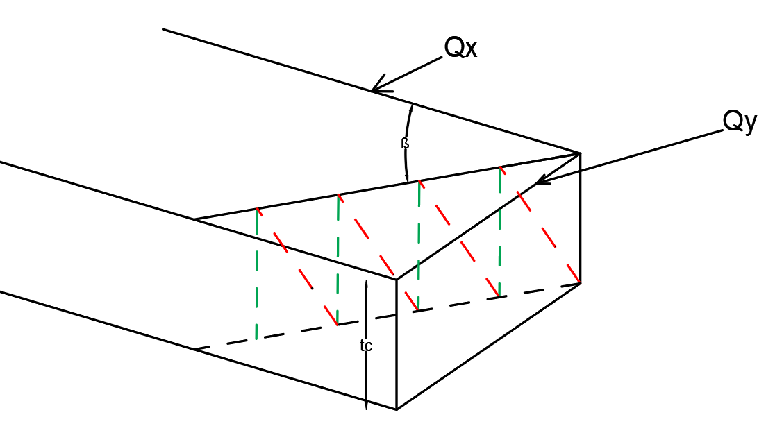
Figure 24.Interlayer reinforcement at the equivalent main shear effort

Moreover, in order to take into account the state of prestress (impact on the coefficients \({\alpha }_{\mathit{cw}}\) and \({\sigma }_{\mathit{cp}}\)), the following are considered as normal calculation effort:

\({N}_{\mathit{Ed}}={N}_{\mathit{xx}}{\mathrm{cos}}^{2}\left(\beta \right)+2{N}_{\mathit{xy}}\mathrm{cos}\left(\beta \right)\mathrm{sin}\left(\beta \right)+{N}_{\mathit{yy}}{\mathrm{sin}}^{2}\left(\beta \right)\)

In the case where the calculation shows that transverse reinforcement is required (\({V}_{\mathit{Ed}0}>{V}_{\mathit{Rd},c}\)) then, in accordance with Eurocode, a reinforcement of design \({A}_{\mathit{sv}0}\) (cm2/ml/ml) is calculated in the direction \(\beta\) and from there, we transition to the “real” transverse reinforcement in order to verify the inequality below:

\({A}_{\mathit{sv},x}{\mathrm{cos}}^{2}\left(\beta \right)+{A}_{\mathit{sv},y}{\mathrm{sin}}^{2}\left(\beta \right)\ge {A}_{\mathit{sv}\mathrm{,0}}\)

(Reasoning similar to that introduced in Capra-Maury)

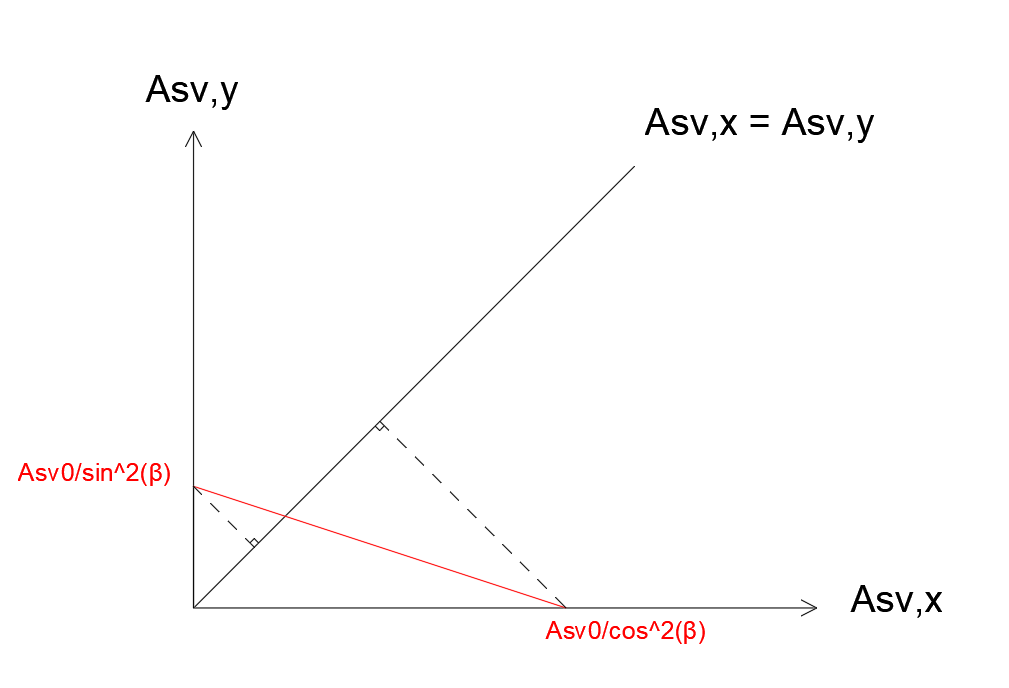
Figure 25 .Finding the optimal transverse reinforcement

Thus, the search for the optimum reinforcement consists in determining the point on the red line, whose projection on the 1st bisector of the plane (Asv, x; Asv, y) is the closest to the origin of the coordinate system. Therefore, the final solution will be:

If \(\beta =0\to {{A}_{\mathit{sv}}}_{x}={{A}_{\mathit{sv}}}_{0}{\mathit{et}{A}_{\mathit{sv}}}_{y}=0\)
If \(\beta =\pm \frac{\pi }{2}\) \(\to {{A}_{\mathit{sv}}}_{x}=0{\mathit{et}{A}_{\mathit{sv}}}_{y}={{A}_{\mathit{sv}}}_{0}\)
If not:
si:math: left|betaright|<frac {pi} {4}, we take:math: {{A} _ {mathit {sv}}}} _ {x}} =frac {{{A} | =frac {{A}} _ {{A} _ {{A} _ {0}}} {{mathrm {cos}}}} _ {cos}}} _ {x} =frac {{A} _ {{A} _ {A} _ {A} _ {A} _ {A} _ {A} _ {2}beta} _ {{A} _ {0}}} {mathrm {cos}}}} ^ {2}beta} {mathit {and} {A} _ {mathit {sv}}}} _ {y} =0
si:math: left|betaright|>frac {pi} {4}, we take:math: {{A} _ {mathit {sv}}}} _ {x}} =0 {mathit {}} =0 {mathit {and} {a} =0 {mathit {and} {a} =0 {mathit {and} {A} =0 {mathit {and} {A} =0 {mathit {and} {A} =0 {mathit {and} {A} =0 {mathit {and} {A} =0 {mathit {and} {A} =0 {mathit {and} {A} =0 {mathit {and} {A} =0 {mathit {and}}} _ {0}} {{mathrm {sin}}} ^ {2}beta}
math:

mathit {si}left|betaright|=frac {pi} {4}, we take:math: {{A} _ {mathit {sv}}}}} _ {x}}} _ {x}} =frac {{{A}} _ {{{A}} _ {0}}} {2 {mathrm {sv}}}} {2 {mathrm {sv}}}}} _ {cos}}} ^ {2}beta} `:math: {mathit {and} {A} _ {mathit {sv}}}} _ {y} =frac {{{A} _ {mathit {sv}}}}}} _ {0}}} {0}}} {0}}} {0}}} {0}}} {{2}beta} `

Moreover, in the case where transverse reinforcement is required, the additional tensile forces introduced at the level of the equations in §2.2.2 of this note must be added:

\({D}_{\mathit{nxx}}=\frac{{Q}_{x}^{2}}{{V}_{\mathit{Ed}0}}\times \mathit{cot\theta }\)

\({D}_{\mathit{nyy}}=\frac{{Q}_{y}^{2}}{{V}_{\mathit{Ed}0}}\times \mathit{cot\theta }\)

\({D}_{\mathit{nxy}}=\frac{{Q}_{x}\times {Q}_{y}}{{V}_{\mathit{Ed}0}}\times \mathit{cot\theta }\)

\(\theta\) being the angle of inclination of the compression rod in the Ritter-Mosche truss for shear reinforcement of the \(\beta\) steering beam.

2.3. Taking into account the minimum reinforcement#

For the minimum percentage of longitudinal steel in the main direction, and in accordance with the specifications in §9.3 of EC2, the specifications in §1.5.1 of this documentation apply.

No minimum threshold is required for cross reinforcement.

2.4. Properties relating to the outlet reinforcement field#

The current version of operator CALC_FERRAILLAGEpropose also calculates the following quantities, after determining the reinforcement field required by the element:

2.4.1. Calculation of reinforcement volume density#

At the end of the calculations at \(\mathit{ELU}/\mathit{ELS}/\mathit{ELSQP}\), the flexural steel sections \({A}_{\mathit{XS}}\), \({A}_{\mathit{XI}}\), \({A}_{\mathit{YS}}\), \({A}_{\mathit{YI}}\) and the shear steel sections \({A}_{\text{sv,x}}\) and \({A}_{\text{sv,y}}\) are used to calculate the reinforcement volume density \({\mathrm{\delta }}_{\mathit{BA}}\) in \(\mathit{kg}/{m}^{3}\) if they are expressed in \({m}^{2}/m\) for flexure steels in \({m}^{2}/{m}^{2}\) for shear steels according to the following formula where \({\mathrm{\rho }}_{\mathit{acier}}\) is the density of steels in \(\mathit{kg}/{m}^{3}\).

\({\mathrm{\delta }}_{\mathit{BA}}=\frac{({A}_{\mathit{XS}}+{A}_{\mathit{YS}}+{A}_{\mathit{XI}}+{A}_{\mathit{YI}})+({A}_{\text{SV,X}}+{A}_{\text{SV,Y}})\ast h}{h}\ast {\mathrm{\rho }}_{\mathit{acier}}\)

2.4.2. Calculation of the constructability complexity indicator#

A complexity indicator aimed at translating the difficulty of implementing reinforcement in the field is calculated according to the following formula:

\({I}_{c,i}=\frac{{\mathrm{\alpha }}_{\mathit{reinf}}\cdot \frac{{\mathrm{\rho }}_{i}}{{\mathrm{\rho }}_{\mathit{critic}}}+{\mathrm{\alpha }}_{\mathit{shear}}\cdot \frac{{A}_{\mathit{sw},i}}{{A}_{\mathit{sw},\mathit{critic}}}+{\mathrm{\alpha }}_{\mathit{stirrups}}\cdot \frac{{A}_{\mathit{sw},i}}{{A}_{\mathit{sw},\mathit{critic}}}\cdot \frac{{h}_{\mathit{eff},i}}{{l}_{\mathit{crit}}}}{{\mathrm{\alpha }}_{\mathit{reinf}}+{\mathrm{\alpha }}_{\mathit{shear}}+{\mathrm{\alpha }}_{\mathit{stirrups}}}\)

With:

\({\mathrm{\alpha }}_{\mathit{reinf}}\) is a weighting factor of the steel density ratio per cubic meter of concrete;

\({\mathrm{\rho }}_{i}\) is the total steel volume density for element i calculated previously \({\mathrm{\delta }}_{\mathit{BA}}\);

\({\mathrm{\rho }}_{\mathit{critic}}\) is the critical steel volume density for element i;

\({\mathrm{\alpha }}_{\mathit{shear}}\) is a weighting coefficient of the shear steel density ration;

\({A}_{\mathit{sw},i}=\sqrt{{A}_{\text{sv,x}}^{2}+{A}_{\text{sv,y}}^{2}}\) is the shear steel density for element i;

\({A}_{\mathit{sw},\mathit{critic}}\) is the critical shear strength reinforcement density;

\({\mathrm{\alpha }}_{\mathit{stirrups}}\) is a weighting factor of the length ratio of shear steel pins;

\({h}_{\mathit{eff},i}=h-c-c\text{'}\) is the effective height considered for element i;

\({l}_{\mathit{crit}}\) is the critical length for shear steel pins.

\({\mathrm{\alpha }}_{\mathit{reinf}}\), \({\mathrm{\alpha }}_{\mathit{shear}}\) and \({\mathrm{\alpha }}_{\mathit{stirrups}}\) have the default value \(1\), the critical steel volume density \({\mathrm{\rho }}_{\mathit{critic}}\) has the default value \(150\mathit{kg}/m\mathrm{³}\), the critical shear reinforcement density \({A}_{\mathit{sw},\mathit{critic}}\) has the default value \(60\mathit{cm}\mathrm{²}/m\mathrm{²}\) and the critical length of the shear steel pins has the default value and the critical length of shear steel pins has the default value \(1m\).

With such values, it is considered that the transition between constructible and unconstructible is given for values of \({l}_{c}\) between \(1\) and \(\mathrm{1,2}\). Beyond \({l}_{c}=2\) we consider that the implementation of reinforcement is very complicated and beyond \({l}_{c}=3\) we consider that the implementation of reinforcement is impossible.