5. Calculation of the shear half-amplitude#
The problem is therefore to find the circle circumscribed to a certain number of points located in a plane. The shear half-amplitude will be equal to the radius of the circumscribed circle.
5.1. Overview of the circumscribed circle calculation#
The method we use is an exact method that is broken down into four steps.
Step 1
We frame the points and we determine the coordinates of the four corners of the frame in the frame \((\mathrm{0,}u,v)\), and the coordinates of the center of the frame \(O\) cf. [Figure 5.1-a] and [Figure 5.1-c]. In the particular case where the frame is reduced to a horizontal or vertical line, the half-length of the line is equal to the half-shear amplitude.
Step 2
The objective of the second stage is to select the two most distant points. In order not to examine the distance between all possible pairs of points, we construct four sectors, cf. [Figure 5.1-a] and [Figure 5.1-c]. These sectors are located at the four corners of the frame and are delimited, on the one hand, by the outline of the frame and, on the other hand, by an arc whose center is the opposite corner and the radius is the long side of the frame, which in fact reduces the distance between the two most distant points. Finally, we evaluate the distances between the points of the four sectors two by two:
distances between the points in sector 1 and the points in sector 2;
distances between the points in sector 1 and the points in sector 3;
distances between the points in sector 1 and the points in sector 4;
distances between the points in sector 2 and the points in sector 3;
distances between the points in sector 2 and the points in sector 4;
distances between the points in sector 3 and the points in sector 4.
In the particular case where the ratio of the short side of the frame to the long side is strictly less than \(\sqrt{3\mathrm{/}4}\) we do not evaluate the distances between the points belonging to sectors 1 and 2 nor the distances between the points of the sectors 3 and 4, case of the example of [Figure 5.1-a].
Step 3
In the third step we build domains 1 and 2 where we will look for points that are outside the initial circumscribed circle, see Step 4. The purpose of creating domains 1 and 2 is to reduce the number of points to be explored during step 4. The principles of construction in these two fields are as follows.
From the midpoints on the two main sides of the frame (\({\text{Omi}}_{1}\) and \({\text{Omi}}_{2}\), cf. [Figure 5.1-b] and, cf. [] and [Figure 5.1-d]) we draw an arc whose radius corresponds to the minor of the value of the half-shear amplitude and is equal to the half-length of the long side of the frame.
From the center of frame \(O\) we draw four arcs whose radius is also the minor of the value of the half-shear amplitude.
If \({O}_{i}\) the center of the initial circumscribed circle has a component along the \(u\) axis that places it between \({\text{Omi}}_{1}\) and \(O\), then if there is a point whose distance to \({O}_{i}\) is greater than \({R}_{i}\) the radius of the initial circumscribed circle, it can only be in domain 1, cf. [Figure 5.1-b].

Figure 5.1-a: Example 1, location of sectors |

Figure 5.1-b: Example 1, location of domains |

Figure 5.1-c: Example 2, location of sectors |

Figure 5.1-d: Example 2, location of domains |
Step 4
The aim of the fourth step is to find the circumscribed circle using the three-point circle method, cf. [§5.2]. To do this, we calculate the midpoint \({O}_{1}\) associated with the two most distant points that we note \({P}_{1}\) and \({P}_{2}\), we deduce the value of a first radius noted as \({R}_{1}\). Depending on the position of \({O}_{1}\) in relation to the major axis of the frame passing through its center, we search either in domain 1 or in field 2, if there is a point located at a distance greater than the half distance measured between the two farthest points \({P}_{1}\) and \({P}_{2}\). Let’s note \({P}_{3}\) such a point. If there is no point such as \({P}_{3}\) then the half-shear amplitude is equal to \({R}_{1}\), cf. [Figure 5.1-c]. On the other hand, if \({P}_{3}\) exists we look for the coordinates of the point located equidistant from \({P}_{1}\), \({P}_{2}\) and \({P}_{3}\); we note this point \({O}_{2}\). We thus obtain a new radius, \({R}_{2}\) and therefore a new half-shear amplitude. Again, depending on the position of \({O}_{2}\) in relation to the major axis of the frame passing through its center, we look either in domain 1 or in field 2, if there is a point located at a distance greater than \({R}_{2}\) from \({O}_{2}\). Let’s note \({P}_{4}\) such a point. If there is no point such as \({P}_{4}\) then the half shear amplitude is equal to \({R}_{2}\). On the other hand, if \({P}_{4}\) exists we look for the smallest circle circumscribed to the four points: \({P}_{1}\), \({P}_{2}\), \({P}_{3}\) and \({P}_{4}\) by successively using the circle method passing through three points, cf. [§5.2]. This provides us with a new \({O}_{3}\) center and a new \({R}_{3}\) radius. As before, depending on the position of \({O}_{3}\) in relation to the major axis of the frame passing through its center, we search either in domain 1 or in field 2, if there is a point located at a distance greater than \({R}_{3}\) from \({O}_{3}\). Let’s note \({P}_{5}\) such a point. If there is no point such as \({P}_{5}\) then the half shear amplitude is equal to \({R}_{3}\). On the other hand, if a point such as \({P}_{5}\) exists we have five points, if we want to use the previous method, where there are only four points in play, it is necessary to eliminate one of the five points. It can’t be the last one: \({P}_{5}\), so we’re keeping from the previous iteration the three points that made it possible to determine \({O}_{3}\) and \({R}_{3}\), i.e. the smallest circumscribed circle. Let’s assume that \({P}_{1}\) is eliminated in this way. We are therefore looking for the smallest circle circumscribed to the four points: \({P}_{2}\), \({P}_{3}\),, \({P}_{4}\) and \({P}_{5}\) by successively using the circle method passing through three points, cf. [§5.2]. This provides us with a new \({O}_{4}\) center and a new \({R}_{4}\) radius. Depending on the position of \({O}_{4}\) in relation to the major axis of the frame passing through its center, we search either in domain 1 or in field 2, if there is a point located at a distance greater than \({R}_{4}\) from \({O}_{4}\). If this is not the case, the half-shear amplitude is equal to \({R}_{4}\) and the circumscribed circle has \({O}_{4}\) as its center, cf. [Figure5.1-f]. Conversely, if such a point exists we repeat an iteration identical to the previous one.
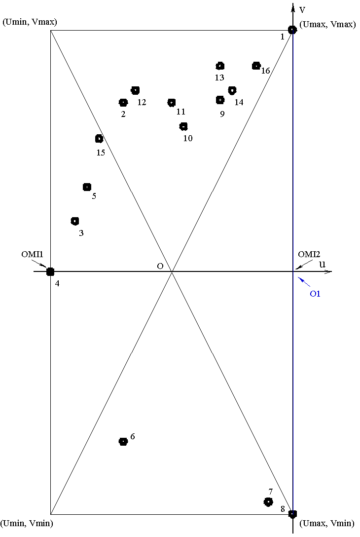
Figure 5.1-e: Example1, finding the circumscribed circle |
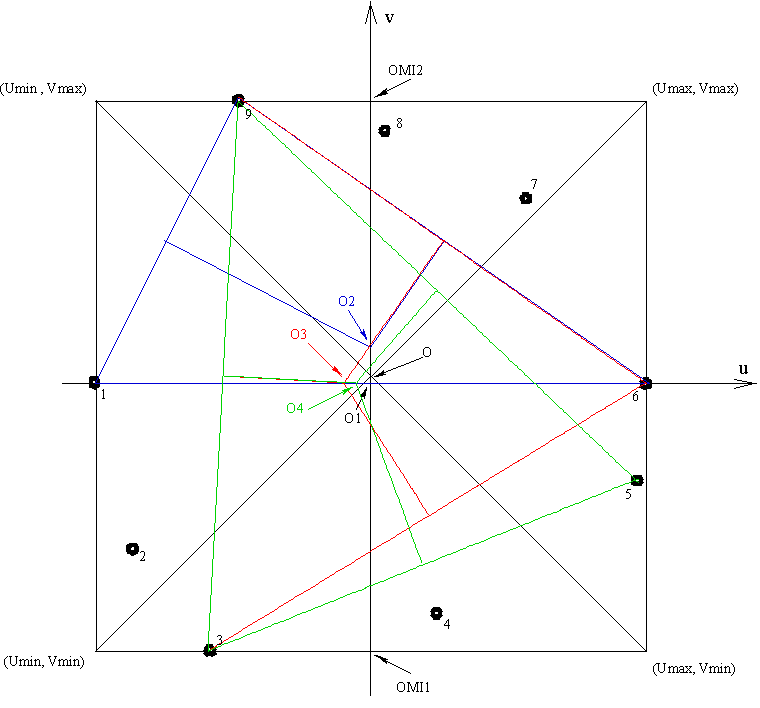
Figure 5.1-f: Example2, finding the circumscribed circle |
5.2. Description of the circle method passing through three points#
In this paragraph we will deal with the general case and then with the specific cases.
5.2.1. General case#
To determine the circle circumscribed at three points \({P}_{0}\), \({P}_{1}\) and \({P}_{2}\), see [Figure 5.2.1-a], we proceed in three steps.

Figure 5.2.1-a: Determining the circle passing through three points
Step 1
We calculate the coordinates of the three midpoints: \({M}_{0}\), \({M}_{1}\) and \({M}_{2}\), cf. [Figure 5.2.1-a].
Step 2
We determine the normals passing through the three midpoints: \({M}_{0}\), \({M}_{1}\) and \({M}_{2}\), cf. [Figure5.2.1-A]. These normals are lines of the type \(v=au+b\) where \(a\) and \(b\) are constants that can be calculated with the coordinates of the points \({P}_{0}\), \({P}_{1}\), \({P}_{2}\), \({M}_{0}\), \({M}_{1}\) and \({M}_{2}\). Let us now describe how to determine these normals.
1) Normal to segment \({P}_{0}\) \({P}_{1}\) going by \({M}_{1}\)
We determine the coordinates of a point \({M}_{1}^{\text{'}}\) by rotating the segment \({P}_{0}\) \({M}_{1}\) by 90°:
\(\begin{array}{c}{U}_{M{1}^{\text{'}}}\mathrm{=}{U}_{\mathit{M1}}+({V}_{\mathit{M1}}\mathrm{-}{V}_{\mathit{P0}})\\ {V}_{M{1}^{\text{'}}}\mathrm{=}{V}_{\mathit{M1}}+({U}_{\mathit{P0}}\mathrm{-}{U}_{\mathit{M1}})\end{array}\) eq 5.2.1-1
where \({U}_{k}\) and \({V}_{k}\) with \(k\mathrm{=}M{1}^{\text{'}},\mathit{M1},\mathit{P0}\) represent the components \(u\) and \(v\) of the points \({M}_{1}^{\text{'}}\), \({M}_{1}\), and \({P}_{0}\). From this we deduce the constants \({a}_{0}\) and \({b}_{0}\) of the line representing the normal to the segment \({P}_{0}\) \({P}_{1}\) passing through \({M}_{1}\):
\(\begin{array}{c}{a}_{0}\mathrm{=}({V}_{M{1}^{\text{'}}}\mathrm{-}{V}_{\mathit{M1}})\mathrm{/}({U}_{M{1}^{\text{'}}}\mathrm{-}{U}_{\mathit{M1}})\\ {b}_{0}\mathrm{=}({U}_{M{1}^{\text{'}}}{V}_{\mathit{M1}}\mathrm{-}{U}_{\mathit{M1}}{V}_{M{1}^{\text{'}}})\mathrm{/}({U}_{M{1}^{\text{'}}}\mathrm{-}{U}_{\mathit{M1}})\end{array}\) eq 5.2.1-2
In the particular case where \(({U}_{\mathit{M1}\text{'}}\mathrm{-}{U}_{\mathit{M1}})\mathrm{=}0\), we force \({a}_{0}\) and \({b}_{0}\) to zero and we get the coordinates of the center \(O\) of the circle circumscribed at the points \({P}_{0}\), \({P}_{1}\), and \({P}_{2}\) by a specific method described in paragraph [§5.2.2].
2) Normal to segment \({P}_{0}\) \({P}_{2}\) going by \({M}_{0}\)
We determine the coordinates of a point \(\mathit{M0}\text{'}\) by rotating the segment \({P}_{0}\) \({M}_{0}\) by 90°:
\(\begin{array}{c}{U}_{\mathit{M0}\text{'}}\mathrm{=}{U}_{\mathit{M0}}+({V}_{\mathit{M0}}\mathrm{-}{V}_{\mathit{P0}})\\ {V}_{\mathit{M0}\text{'}}\mathrm{=}{V}_{\mathit{M0}}+({U}_{\mathit{P0}}\mathrm{-}{U}_{\mathit{M0}})\end{array}\) eq 5.2.1-3
where \({U}_{k}\) and \({V}_{k}\) with \(k\mathrm{=}\mathit{M0}\text{'},\mathit{M0},\mathit{P0}\) represent the components \(u\) and \(v\) of the points \(\mathit{M0}\text{'}\), \({M}_{0}\), and \({P}_{0}\). From this we deduce the constants \({a}_{1}\) and \({b}_{1}\) of the line representing the normal to the segment \({P}_{0}\) \({P}_{2}\) passing through \({M}_{0}\):
\(\begin{array}{c}{a}_{1}\mathrm{=}({V}_{\mathit{M0}\text{'}}\mathrm{-}{V}_{\mathit{M0}})\mathrm{/}({U}_{\mathit{M0}\text{'}}\mathrm{-}{U}_{\mathit{M0}})\\ {b}_{1}\mathrm{=}({U}_{\mathit{M0}\text{'}}{V}_{\mathit{M0}}\mathrm{-}{U}_{\mathit{M0}}{V}_{\mathit{M0}\text{'}})\mathrm{/}({U}_{\mathit{M0}\text{'}}\mathrm{-}{U}_{\mathit{M0}})\end{array}\) eq 5.2.1-4
In the particular case where \(({U}_{\mathit{M0}\text{'}}\mathrm{-}{U}_{\mathit{M0}})\mathrm{=}0\), we force \({a}_{1}\) and \({b}_{1}\) to zero and we get the coordinates of the center \(O\) of the circle circumscribed at the points \({P}_{0}\), \({P}_{1}\), and \({P}_{2}\) by a specific method described in paragraph [§5.2.2].
3) Normal to segment \({P}_{1}\) \({P}_{2}\) going by \({M}_{2}\)
We determine the coordinates of a point \({M}_{2}^{\text{'}}\) by rotating the segment \({P}_{1}\) \({M}_{2}\) by 90°:
\(\begin{array}{c}{U}_{\mathit{M2}\text{'}}\mathrm{=}{U}_{\mathit{M2}}+({V}_{\mathit{M2}}\mathrm{-}{V}_{\mathit{P1}})\\ {V}_{M{2}^{\text{'}}}\mathrm{=}{V}_{\mathit{M2}}+({U}_{\mathit{P1}}\mathrm{-}{U}_{\mathit{M2}})\end{array}\) eq 5.2.1-5
where \({U}_{k}\) and \({V}_{k}\) with \(k\mathrm{=}\mathit{M2}\text{'},\mathit{M2},\mathit{P1}\) represent the components \(u\) and \(v\) of the points \({M}_{2}^{\text{'}}\), \({M}_{2}\), and \({P}_{1}\). From this we deduce the constants \({a}_{2}\) and \({b}_{2}\) of the line representing the normal to the segment \({P}_{1}\) \({P}_{2}\) passing through \({M}_{2}\):
\(\begin{array}{}{a}_{2}=({V}_{M{2}^{\text{'}}}-{V}_{\mathrm{M2}})/({U}_{M{2}^{\text{'}}}-{U}_{\mathrm{M2}})\\ {b}_{2}=({U}_{M{2}^{\text{'}}}{V}_{\mathrm{M2}}-{U}_{\mathrm{M2}}{V}_{M{2}^{\text{'}}})/({U}_{M{2}^{\text{'}}}-{U}_{\mathrm{M2}})\end{array}\) eq 5.2.1-6
In the particular case where \(({U}_{\mathit{M2}\text{'}}\mathrm{-}{U}_{\mathit{M2}})\mathrm{=}0\), we force \({a}_{2}\) and \({b}_{2}\) to zero and we get the coordinates of the center \(O\) of the circle circumscribed at the points \({P}_{0}\), \({P}_{1}\), and \({P}_{2}\) by a specific method described in paragraph [§5.2.2].
Step 3
In the general case, we deduce from the constants \({a}_{0}\), \({b}_{0}\), \({a}_{1}\),,, \({b}_{1}\), \({a}_{2}\) and \({b}_{2}\) the coordinates of the center \(O\) of the circle circumscribed at the points \({P}_{0}\), \({P}_{1}\) and \({P}_{2}\) in three different ways. Let’s note \({O}_{0}\), \({O}_{1}\), and \({O}_{2}\) the same center \(O\), obtained in three different ways, and \({U}_{k}\) and \({V}_{k}\), where \(k={O}_{0},{O}_{1},{O}_{2}\), represent the \(u\) and \(v\) components of the points \({O}_{0}\), 11.0, and \({O}_{1}\) \({O}_{2}\):
\(\begin{array}{}{U}_{{O}_{0}}=({b}_{1}-{b}_{0})/({a}_{0}-{a}_{1})\\ {V}_{{O}_{0}}=({a}_{0}{b}_{1}-{a}_{1}{b}_{0})/({a}_{0}-{a}_{1})\end{array}\) eq 5.2.1-7
\(\begin{array}{}{U}_{{O}_{1}}=({b}_{2}-{b}_{0})/({a}_{0}-{a}_{2})\\ {V}_{{O}_{1}}=({a}_{0}{b}_{2}-{a}_{2}{b}_{0})/({a}_{0}-{a}_{2})\end{array}\) eq 5.2.1-8
\(\begin{array}{}{U}_{{O}_{2}}=({b}_{2}-{b}_{1})/({a}_{1}-{a}_{2})\\ {V}_{{O}_{2}}=({a}_{1}{b}_{2}-{a}_{2}{b}_{1})/({a}_{1}-{a}_{2})\end{array}\) eq 5.2.1-9
After verifying that the equalities: \({U}_{{O}_{0}}\equiv {U}_{{O}_{1}}{U}_{{O}_{2}}\) and \({V}_{{O}_{0}}\equiv {V}_{{O}_{1}}{V}_{{O}_{2}}\) are satisfied we determine the radius of the circumscribed circle by calculating the distance between \(O\) and one of the three points \({P}_{0}\), \({P}_{1}\) or \({P}_{2}\).
5.2.2. Special cases#
In this paragraph we deal with the three specific cases from step 2 of paragraph [§5.2.1].
Special case wher \(({U}_{M{1}^{\text{'}}}-{U}_{\mathrm{M1}})=0\)
In this case we immediately obtain the components \(u\) and \(v\) from the center \(O\) by:
\(\begin{array}{}{U}_{O}={U}_{\mathrm{M1}}\\ {V}_{O}=({a}_{1}{b}_{2}-{a}_{2}{b}_{1})/({a}_{1}-{a}_{2})\end{array}\) eq 5.2.2-1
Special case wher \(({U}_{M{0}^{\text{'}}}-{U}_{\mathrm{M0}})=0\)
Here the components \(u\) and \(v\) of the \(O\) center are given by:
\(\begin{array}{}{U}_{0}={U}_{\mathrm{M0}}\\ {V}_{O}=({a}_{0}{b}_{2}-{a}_{2}{b}_{0})/({a}_{0}-{a}_{2})\end{array}\) eq 5.2.2-2
Special case wher \(({U}_{M{2}^{\text{'}}}-{U}_{\mathrm{M2}})=0\)
In the latter case, the \(u\) and \(v\) of the \(O\) center are given by:
\(\begin{array}{c}{U}_{0}\mathrm{=}{U}_{\mathit{M2}}\\ {V}_{O}\mathrm{=}({a}_{0}{b}_{1}\mathrm{-}{a}_{1}{b}_{0})\mathrm{/}({a}_{0}\mathrm{-}{a}_{1})\end{array}\) eq 5.2.2-3
The value of the radius of the circumscribed circle is obtained in the same way as in the general case; that is, by calculating the distance between \(O\) and one of the three points \({P}_{0}\), \({P}_{1}\), or \({P}_{2}\).
5.3. Criteria with critical plans#
In this paragraph we give the list of criteria with critical plans, cf. [bib3], which are programmed as well as a brief description.
Rating:
\(n\ast\) |
: normal to the plane in which the shear amplitude is maximum; |
\(\Delta \tau (n)\) |
: shear amplitude in a plane with normal \(\overrightarrow{n}\); |
\({N}_{\text{max}}(n)\) |
: maximum normal stress on the plane of normal \(\overrightarrow{n}\) during the cycle; |
\({\tau }_{0}\) |
: endurance limit in pure alternating shear; |
\({d}_{0}\) |
: endurance limit in pure alternating traction-compression; |
\({N}_{m}(n)\) |
: average normal stress on the plane of normal \(\overrightarrow{n}\) during the cycle; |
\({\varepsilon }_{\text{max}}(n)\) |
: maximum normal deformation on the plane of normal \(\overrightarrow{n}\) during the cycle; |
\({\varepsilon }_{m}(n)\) |
: mean normal deformation at the level of normal \(\overrightarrow{n}\) during the cycle; |
\(P\) |
: hydrostatic pressure; |
\({c}_{p}\) |
: harmful effect of pre-work hardening in controlled deformation, \({c}_{p}\ge 1\). |
Criteria of MATAKE
\(\frac{\Delta \tau (n\mathrm{\ast })}{2}+a{N}_{\text{max}}(n\mathrm{\ast })\mathrm{\le }b\) eq 5.3-1
where \(a\) and \(b\) are two constants given by the user, they depend on the material characteristics and are equal to:
\(a\mathrm{=}({\tau }_{0}\mathrm{-}\frac{{d}_{0}}{2})\mathrm{/}\frac{{d}_{0}}{2}b\mathrm{=}{\tau }_{0}\text{.}\)
In addition, we define an equivalent constraint in the sense of MATAKE, noted \({\sigma }_{\text{eq}}(n\mathrm{\ast })\):
\({\sigma }_{\text{eq}}(n\mathrm{\ast })\mathrm{=}({c}_{p}\frac{\Delta \tau (n\mathrm{\ast })}{2}+a{N}_{\text{max}}(n\mathrm{\ast }))\frac{f}{t},\)
where \(f\mathrm{/}t\) represents the ratio of the alternating flexure and torsional endurance limits.
Criteria of DANG VAN
\(\frac{\Delta \tau (n\mathrm{\ast })}{2}+aP\mathrm{\le }b\) eq 5.3-2
where \(a\) and \(b\) are two constants given by the user, they depend on the material characteristics and are equal to:
\(a\mathrm{=}\frac{3}{2}\mathrm{\times }\frac{(\Delta {\sigma }_{2}\mathrm{-}\Delta {\sigma }_{1})}{(\Delta {\sigma }_{1}\mathrm{-}\Delta {\sigma }_{2})\mathrm{-}2{\sigma }_{m}}b\mathrm{=}\frac{{\sigma }_{m}}{(\Delta {\sigma }_{2}\mathrm{-}\Delta {\sigma }_{1})+2{\sigma }_{m}}\mathrm{\times }\frac{\Delta {\sigma }_{1}}{2}\text{.}\)
In addition, we define an equivalent constraint in the sense of DANG VAN, denoted by \({\sigma }_{\text{eq}}(n\mathrm{\ast })\):
\({\sigma }_{\text{eq}}(n\mathrm{\ast })\mathrm{=}({c}_{p}\frac{\Delta \tau (n\mathrm{\ast })}{2}+aP)\frac{c}{t}\),
where \(c\mathrm{/}t\) represents the ratio of alternating shear and tensile endurance limits.
5.4. Number of cycles at breakage and damage#
From \({\sigma }_{\text{eq}}(n\mathrm{\ast })\) and a Wöhler curve we deduce the number of cycles at break: \(N(n\mathrm{\ast })\), then the damage corresponding to one cycle: \(D(n\mathrm{\ast })\mathrm{=}1\mathrm{/}N(n\mathrm{\ast })\).