2. Search for the crack path#
2.1. Generalities#
It is assumed that the crack belongs to a certain group of elements (GROUP_MA), on which field \(X\) (damage, plastic deformation) is defined. The crack is identified by an area where the values in this field are especially high, and normally greater than a certain value: damage greater than \(0\) for example.
In the following, the procedure for finding the crack path is described. We exploit the fact that, in the plane orthogonal to the crack, field \(X\) has a maximum on the crack itself. The procedure is step-by-step, with each step a new crack point is found. It can be described by the not-type, by its initiation and by the stopping criteria.
2.2. Not typical#
At each stage, research requires two points. The last point found \({P}_{i}\) is the starting point and the vector \(\overrightarrow{{P}_{i\mathrm{-}1}{P}_{i}}\) (\({P}_{i\mathrm{-}1}\) being the penultimate point found) gives the search direction.
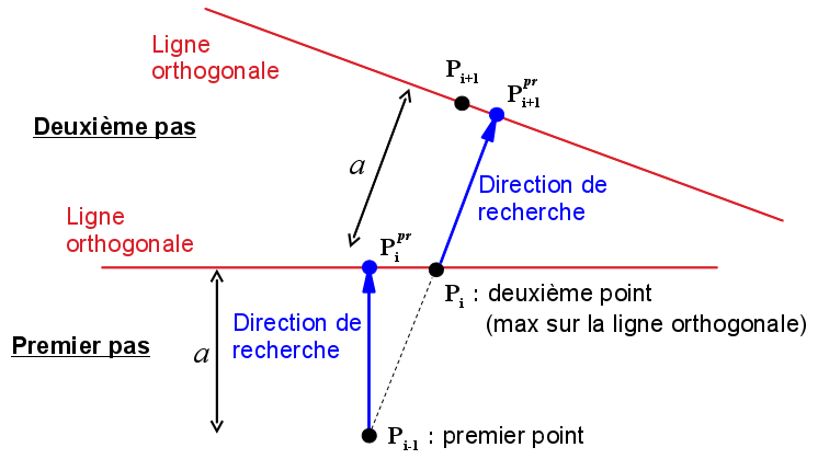
Figure 1: Diagram of the pass type
At each typical step, the following actions are executed (see also the diagram of):
the position of the next point is first estimated (prediction point \({P}_{i}^{\mathit{pr}}\)) at the distance \(a\) from the starting point in the search direction, \(a\) being the no progress;
field \(X\) is projected onto a line orthogonal to the search direction and passing through the prediction point;
the projected field is smoothed by convolution (eq) to partially get rid of the mesh (for example, if we rely on finite elements with linear interpolation, the projected field is linear in pieces);
the new point in crack \({P}_{i+1}\) is where the smoothed field reaches its maximum value.
The smoothing mentioned in point 3 is necessary: for example, if the field projected onto the orthogonal profile is linear in pieces, its maximum is necessarily on the edge of an element. The smoothing is achieved by convolution:
\(\overline{X}(s)\mathrm{=}\frac{{}_{{l}_{\mathit{orth}}}\mathrm{\int }X(\zeta )\Psi (\mathrm{\mid }\zeta \mathrm{-}s\mathrm{\mid })d\zeta }{{}_{{l}_{\mathit{orth}}}\mathrm{\int }\Psi (\mathrm{\mid }\zeta \mathrm{-}s\mathrm{\mid })d\zeta }\) eq 2.2-1
where \(\overline{X}\) is the smoothed field, \({l}_{\mathit{orth}}\) is the length of the line orthogonal to the search direction, \(s\) is the curvilinear abscissa on this line, and \(\Psi\) is a Gauss function:
\(\Psi (\mathrm{\mid }\zeta \mathrm{-}s\mathrm{\mid })\mathrm{=}\mathrm{exp}(\mathrm{-}{(\frac{2(\zeta \mathrm{-}s)}{{l}_{\mathit{reg}}})}^{2})\) eq 2.2-2
An example of fields \(X\) and \(\overline{X}\) based on the parameter \({l}_{\mathit{reg}}\) is given in.
Figure 2: Smoothing field \(X\) projected onto the orthogonal line.
An additional parameter is given by the number of points on the orthogonal line, \({N}_{\mathit{orth}}\). This determines the precision of the discrete convolution product, as well as the \({\delta }_{\mathit{orth}}\mathrm{=}{l}_{\mathit{orth}}\mathrm{/}{N}_{\mathit{orth}}\) precision (distance between points).
Discrete convolution is performed by the convolve function from the numpy python library. The functions s \(X(s)\) and \(\Psi (s)\) are sampled over \({l}_{\mathit{orth}}\) at the constant distance \({\delta }_{\mathit{orth}}\). By calling \(\mathrm{X}\), \(\Psi\) the two sampled vectors, the point \(\overline{{X}_{j}}\) of the vector \(\overline{\mathrm{X}}\) that approximates the smoothed function \(\overline{X}(s)\) by points will be given by:
\(\overline{{X}_{j}}\mathrm{=}\frac{\mathrm{\sum }_{i}{\Psi }_{i}{X}_{i+j}}{\mathrm{\sum }_{i}{\Psi }_{i}}\) eq 2.2-3
2.3. Initialization#
The purpose of initialization is to get the first two points, to continue after as described in the pas-type. A diagram of the initialization procedure is given in:
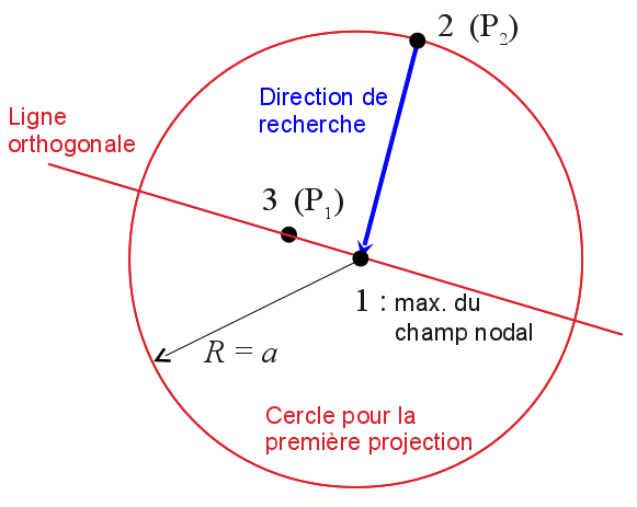
Figure 3: diagram of the initialization procedure.
In detail:
field \(X\) is projected onto a circle with radius \(a\) and centers on node \(1\) where the field at the nodes has its maximum on the chosen GROUP_MA;
field \(X\) is smoothed over the circle via a discrete convolution product (eq.), the second point of the crack \({P}_{2}\) is the point in the circle where \(\overline{X}\) is maximum;
the position of the point \(1\) is corrected by projecting and smoothing the field \(\overline{X}\) on a line orthogonal to \(\overrightarrow{{P}_{2}1}\) and going through \({P}_{2}\): the new point \(3={P}_{1}\) is found;
two possible research directions are thus determined: \(\overrightarrow{{P}_{1}{P}_{2}}\) and \(\overrightarrow{{P}_{2}{P}_{1}}\).
2.4. Stop criteria#
The search for the crack path is completed in both directions \(\overrightarrow{{P}_{1}{P}_{2}}\) and \(\overrightarrow{{P}_{2}{P}_{1}}\) until stopped, in one of the following cases:
the value of the field corresponding to the new point is less than a threshold value, defined a priory. This value must be entered among the command parameters under the BORNE_MIN operand of the RECHERCHE factor keyword.
the prediction point is outside the subject.
2.5. Fields for the search for the crack path#
The method described can be applied to all scalar fields that represent the cracking of the material. Typically, damage \(d\) can be used.
Sometimes the damage field is too « flat », and it breaks a plateau with \(d\mathrm{=}1\). As there would then not be a well-defined maximum, the procedure described in paragraphs 2.2 - 2.3 may not give the desired results. It is then possible to choose other relevant fields: a main deformation component, an equivalent deformation…
An example of choosing the relevant field is given by the test cases zzzz264b, c [V1.01.264].