6. Implemented in Code_Aster#
The mechanical calculation is carried out under the hypothesis of thermo-elasto-plastic behavior associated with a Von Mises criterion with isotropic or linear kinematic hardening (VMIS_ISOT_TRAC, VMIS_ISOT_LINE, VMIS_CINE_LINE). We will specify what the calculation of \({G}_{p}\) consists of and how to identify the material parameters \(R=D/2\) (radius of the cut) and \({G}_{\mathit{pc}}\) (break limit).
The methodology for calculating and identifying with Code_Aster is presented in [U2.05.08]. The easy to use documentation is in [U4.82.31].
6.1. Gp calculation#
The calculation of \({G}_{p}\), carried out using the CALC_GP macro command, is based on the use of POST_ELEM which allows the calculation of elastic energy on a group of elements. The models (finite elements, small deformations, etc.) and loads that can be used are those of the command POST_ELEM, keyword ENER_ELTR. More precisely, for each moment provided in the list of calculation moments, it is a question of carrying out the following two steps:
1/ First calculate quantity \(\stackrel{~}{{G}_{p}}(\mathrm{\Delta }a)\) for increasing values of \(\mathrm{\Delta }a\) by:
\(\stackrel{~}{{G}_{p}}(\mathrm{\Delta }a)=\frac{{\int }_{\mathrm{\Omega }}{\mathrm{\Phi }}_{t}^{\mathit{el}}d\mathrm{\Omega }}{\mathrm{\Delta }a}\)
In 2D, it is therefore necessary to identify the elements of zone \(C\left(\mathrm{\Delta }a\right)\) by a group of elements defined at the level of the mesh as presented in [Figure 2-a], or by a geometric zone of Gauss points, then calculate the elastic energy on this zone and then divide it by \(\mathrm{\Delta }a\).
To identify the elements of zone \(C\left(\mathrm{\Delta }a\right)\), we will proceed as follows: the elements of the first chip will constitute a first group of elements, the elements of chips 1 and 2 will constitute a second group, the elements of chips \(\mathrm{1,}\mathrm{2,}\mathrm{3,}\mathrm{...},i\) will constitute a \(i\) th group, etc. We must provide a number of chips large enough to be able to find the maximum of \(\stackrel{~}{{G}_{p}}(\mathrm{\Delta }a)\), which is most often located at a distance of approximately \(3R\) from the bottom of the notch.
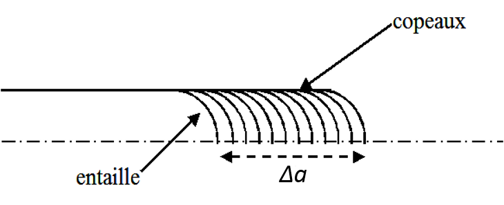
Figure 6.1-1- Definition of chips in the mesh
2/ Then it is a question of identifying the maximum of this function:
\({G}_{p}=\underset{\mathrm{\Delta }a}{\mathit{max}}\stackrel{~}{{G}_{p}}(\mathrm{\Delta }a)\)
Examples and usage tips can be found in document [:ref:` U2.05.01 < U2.05.01 >`], in the ssnp131 tests (see [V6.03.131] and ssnv218 (see [V6.04.218]).
6.2. Identifying parameters#
The energy model is based on the pair of material parameters \(({G}_{\mathit{pc}},R)\), which must therefore be determined at each temperature. Note that \({G}_{\mathit{pc}}\) actually depends on the notch radius [WAD 13]. We will see that the prediction of the breakup does not depend on it.
On the one hand, the Young modulus \(E\) and the critical stress \({\sigma }_{c}\) of a material are assumed to be known. On the other hand, it is hypothesized to know toughness \({K}_{\mathit{Jc}}\) evaluated experimentally from a tensile test on a CT specimen, for example. The application of the « minimum in relation to damage » at the scale of a material point in a state of simple tensile stress gives the relationship between the energy volume dissipated by a material point that is damaged \({w}_{c}\) and the critical stress [WAD 13] (hypothesis H11):
We then obtain the following equation which must be solved in order to identify the two parameters:
: label: eq-25
{G} _ {mathit {pc}} (R) =frac {{mathrm {sigma}} _ {c} ^ {2}} {2}} {E}} R
Left-hand member \({G}_{\mathit{pc}}\left(R\right)\) is a nonlinear function of \(R\). The right-hand side is a linear function of \(R\). Thus, to solve (25) it is necessary to calculate \({G}_{\mathit{pc}}\) for different values of \(R\) as illustrated in figure [Figure 6.2-1].
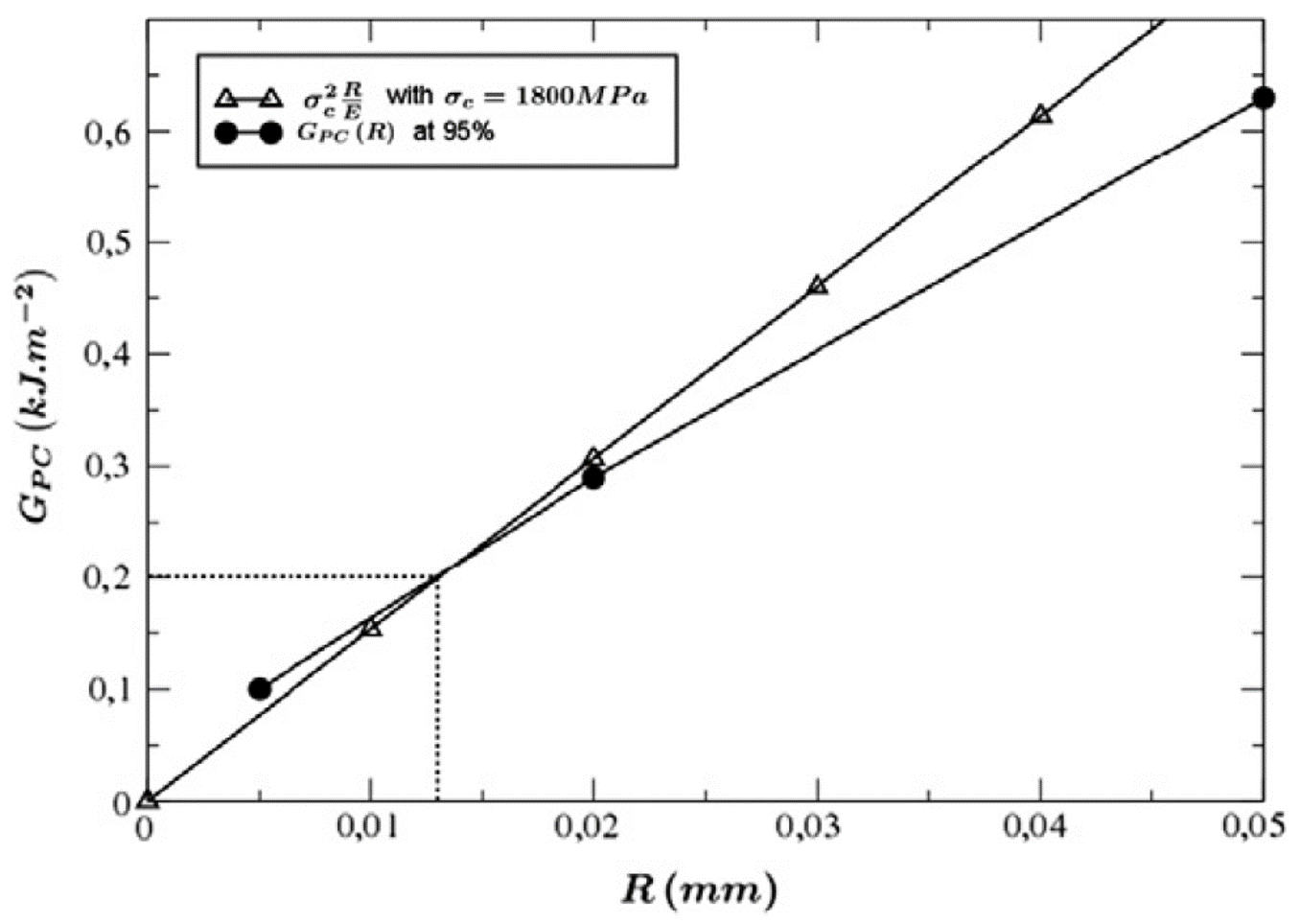
Figure 6.2-1: identifying the \(({G}_{\mathit{pc}},R)\) couple [WAD 13]
For each notch with a given radius \(R\), the parameter \({G}_{\mathit{pc}}\) is determined by simulating a test on a test specimen \(\mathit{CT}\) in the following manner: for each value of the load, increasing from 0 to a critical value, the parameter \({K}_{J}\) is calculated on the one hand and the parameter \({G}_{p}\) on the other hand is calculated. For the critical load value corresponding to \({K}_{J}={K}_{\mathit{Jc}}\), we get \({G}_{p}={G}_{\mathit{pc}}\) (Hypothesis H12).
Solving equation (25) for various values of \(R\) finally makes it possible to determine both the value of \(R\) and the value of \({G}_{\mathit{pc}}\) at a given temperature. In the case of steel, values between 10 and 100 microns are found, which is representative of a real crack.