3. Continuous equations#
3.1. Mechanics#
3.1.1. Constitutive equations#
The formulation of cohesive zone models and their numerical integration are presented in the reference documentation [R7.02.11]. This is a very brief reminder of this.
We are looking for the field of displacement \(u\) at equilibrium by minimizing energy
where \(\phi\) is the density of mechanical energy by volume, \({W}^{\text{ext}}\) is the work of external forces, and \(\Psi\) is the density of surface energy.
The data in \(\Psi\) characterizes the mechanical behavior of the interface. It is expressed by a cohesive law that relates the cohesive force \(\tau\) that is exerted on the lips of the crack to the displacement jump by:
Moreover, the hypothesis of effective constraints is made. In the massif, the total stress tensor is broken down into:
where \(\sigma \text{'}\) refers to the effective stress and \({\sigma }_{p}\) to the hydraulic stress.
On the discontinuity, the total stress vector is decomposed into:
where \(\tau \text{'}\) refers to the effective constraint.
3.1.2. Laws of behavior#
3.1.2.1. Effective constraints#
In the massif, the hypothesis of effective Biot constraints for saturated environments is made, by introducing the hydraulic stress \({\sigma }_{p}\) as a function of the pressure \(p\) (in this case \({p}^{\text{+}}\) or \({p}^{\text{-}}\) in the massif) such that:
where \(b\) is the Biot coefficient of the material.
On discontinuity, within the framework of a cohesive zone model, three zones are distinguished:
an open area where the total stress on the lips is equal to \(pn\);
a transition zone between the open environment and the healthy environment. In this zone, the appearance of micro-cracking and plasticity is observed. The plastic incompressibility of the matrix is thus hypothesized and it is the effective Terzaghi stress that controls the opening of the zone. The total constraint is then written
a healthy area where there is adhesion and no interpenetration of the lips. As long as the stress value remains less than the critical stress, the opening remains zero.
We therefore make the hypothesis, consistent with the behavior of these three zones, that
3.1.2.2. Cohesive laws#
The model presented here is compatible with cohesive laws whose energy is regulated at zero:
CZM_LIN_REG,
CZM_EXP_REG.
These laws make it possible to take into account:
The non-interpenetration of the crack lips by penalization;
The propagation of cracks by a softening law;
The irreversibility of cracking.
The material parameters of the interface are the critical stress at break \({\sigma }_{c}\) and the rupture energy \({G}_{c}\). The numerical parameters are the energy regularization parameter PENA_ADHERENCE and the interpenetration penalization parameter PENA_CONTACT.
3.1.2.3. Bandis law#
In this case, the joint model does not take crack propagation into account. The joint separates two massive bodies by being open all the way and is simply equipped with a law that links the opening to the effective stress.
In the case of Bandis’s empirical law, the relationship between normal effective stress \(\tau {\text{'}}_{n}\) and normal crack closure \(U={U}_{\text{max}}-\varepsilon\) (where \(U\) denotes \(〚u〛\mathrm{.}n\)) is given by
where \({U}_{\mathrm{max}}\) is the asymptotic closure of the crack, \({K}_{\text{ni}}\) is the normal initial stiffness of the discontinuity, and \(\gamma\) is an empirical coefficient that varies between 2 and 6 and depends on the roughness of the walls of the joint. The law of behavior () is shown in figure.
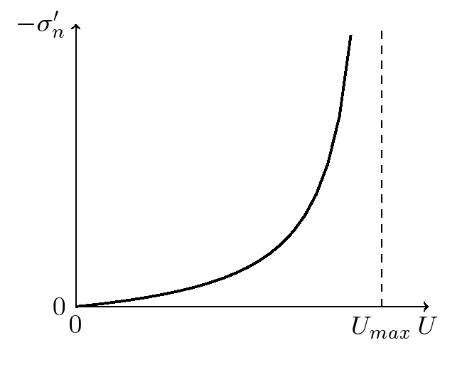
Illustration 3.1.1: Goodman’s law: stress-closure curve
In the tangential direction, the behavior is assumed to be elastic.
The Code_Aster keyword corresponding to this law is JOINT_BANDIS. This keyword should be entered in DEFI_MATERIAU as well as in the behavior (in RELATION_KIT).
3.2. Hydraulics#
3.2.1. Constitutive equations#
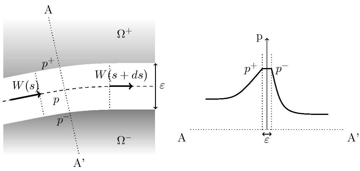
Figure 3.2.1: mass conservation in the crack (left) and typical pressure profile across the interface (right)
The equation for the conservation of mass in the crack is written as
Since the crack thickness is small, it is considered that the pressure field is continuous across the interface. At every point of the interface, we therefore have
On the other hand, flow discontinuities are allowed across the interface (see figure right)
3.2.2. Laws of behavior#
The mass contributions of fluid in the open crack are written as
Where \(\rho\) is the density of the fluid.
The evolution of mass inputs is given by:
where \({K}_{f}\) is the compressibility module of the fluid and \(N\) is the Biot module of the cohesive zone.
The flow in the crack is considered to be darceal. Mass flow can therefore be written as
where \({\lambda }_{H}\) is the hydraulic conductivity of the crack and z refers to the coordinate along the vertical axis. It is given by
The relationship between flow and pressure gradient is given by cubic law. The volume flow through the crack is then written
and intrinsic permeability \(K\) as a function of openness
Note \(T\) the transmittance of the crack, defined by
This law is found analytically by Poiseuille’s law when studying a laminar flow between two smooth plates separated by a distance \(\varepsilon\) that is small compared to the other dimensions. Its validity has also been demonstrated on cracks in rocks for a wide range of parameters.
When the crack walls are impermeable, the mass can be modelled with conventional mechanical finite elements. In this case, the flow equation becomes singular in the closed and undamaged crack portion. A regularization parameter OUV_FICT is therefore introduced which makes it possible to have a fictitious flow in the closed crack portion. On closed elements, we take \(\varepsilon\) equal to OUV_FICT.